SPARX: An Open-Source, Automated, Programmatically Generated, Frequency-Scalable Six-Port Receiver in 130-nm CMOS

This repository requires the IIC-OSIC-TOOLS container with tag 2026.10 or later. All commands below run inside the container, from the repository root. 2026.10 is the first image with the VACASK and snp2le that the noise benches and the thermal-noise fit need, see Section 3.1.
The design and the flow are described in a paper accepted for publication at the 2026 IEEE Nordic Circuits and Systems Conference (NorCAS) (Dorrer et al. 2026). This documentation follows the repository and carries more derivations and results than the paper. We happily accept pull requests and issues.
© 2026 IEEE. Personal use of this material is permitted. Permission from IEEE must be obtained for all other uses, in any current or future media, including reprinting/republishing this material for advertising or promotional purposes, creating new collective works, for resale or redistribution to servers or lists, or reuse of any copyrighted component of this work in other works.
1 Overview
SPARX stands for Six-Port Automated Receiver (RX). It is a mm-wave six-port receiver in the 130 nm IHP SG13CMOS technology whose complete layout is generated by one Python script from a single input, the design frequency. The default design frequency is 160 GHz in the D-band, and the same script generates layouts from 60 GHz to 300 GHz. A 160 GHz receiver was taped out on an IHP open MPW run in March 2026, and the bare dies are back from fabrication (Figure 17).
The name carries a second meaning: SPARX sounds like spark, which is Funken in German, and the German verb funken means to communicate by radio.
The project has three parts:
- A chip. A passive six-port core of one hairpin coupled-line bandpass filter (BPF), one Wilkinson power divider (WPD) and three branch-line couplers (BLC), built as embedded microstrip on TopMetal2 over a Metal5 ground plane, followed by four Schottky barrier diode (SBD) power detectors. It uses CMOS devices only, so it needs no heterojunction bipolar transistor (HBT) as earlier mm-wave six-ports did (Laemmle et al. 2013; Voelkel et al. 2018).
- A flow. Layout generation with GDSFactory and a custom IHP Open-PDK add-on, DRC, LVS and PEX with KLayout, Magic and Netgen, EM simulation with AWS Palace, lumped-element (LE) models of the EM results with snp2le, and circuit simulation with ngspice and VACASK, all driven by one
Makefileinside the IIC-OSIC-TOOLS container. - A characterization. The detector and the complete post-layout receiver are characterized in VACASK with harmonic balance (HB), periodic steady state (PSS) by shooting, their small-signal and noise extensions (HBAC, HBNOISE, PAC, PNOISE), and transient noise (TN). Except for HB, VACASK gained these analyses in 2026, after the tapeout.
The video shows the generation of thirteen receivers from 60 GHz to 300 GHz in 20 GHz steps, which takes less than one minute.
Index Terms: Branch-line coupler, CMOS-only, frequency-scalable layout, GDSFactory, hairpin coupled-line bandpass filter, IHP Open-PDK, large-signal noise, mm-wave, open-source EDA, power detector, programmatic layout, Schottky barrier diode, six-port receiver, Wilkinson power divider.
1.1 Chip Specifications
| Parameter | Value |
|---|---|
| Technology | IHP SG13CMOS, 130 nm CMOS, open-source collateral of the ihp-sg13g2 PDK |
| Design frequency | 160 GHz as taped out, 60 GHz to 300 GHz from the generator |
| Die area | 1 × 1.4 mm² |
| Supply voltage | 1.5 V |
| RF metal stack | TopMetal2 signal lines over a Metal5 ground plane, \(\varepsilon_\mathrm{r} = 4.1\) |
| Six-port core | 1 BPF (third-order Butterworth, hairpin), 1 WPD (no isolation resistor), 3 BLC, 52 \(\Omega\) termination |
| Detectors | 4 forward-biased SBD power detectors with transimpedance amplifier (TIA) and replica |
| RF and LO inputs | ground-signal-ground probe pads |
| Supply and detector outputs | bond pads for PCB bonding |
| Tapeout | IHP open MPW, March 2026, cell RFFE6027 |
1.2 Simulated Performance at a Glance
All numbers are simulated, at the typical corner and 27 °C, with VACASK. Silicon has not been measured yet, see Section 13.
| Quantity | Value | Section |
|---|---|---|
| Detector responsivity, fabricated (\(m = 1\)) | 41 V/W, flat from -71 dBm to -8 dBm | Section 6.3 |
| Detector 1 dB compression, fabricated | -2.7 dBm | Section 6.3 |
| Detector coupling efficiency, fabricated | 0.25 % | Section 6.3 |
| Detector NEP at 1 GHz video frequency, fabricated | 226 pW/\(\sqrt{\text{Hz}}\) | Section 6.4 |
| Detector double-sideband NF at 2 GHz IF, minimum over LO power | 42.3 dB fabricated, 42.7 dB post-layout, 26.8 dB with 16 cells | Section 6.4 |
| LO path loss into the post-layout detectors | 17.3 dB to 18.6 dB | Section 11 |
| RF path loss into the post-layout detectors | 5.4 dB to 9.3 dB | Section 11 |
| I/Q amplitude imbalance and phase difference, post-layout receiver | 2.0 dB and 85.4° | Section 11 |
| Receiver NF at 2 GHz IF, post-layout, I and Q outputs | 48.5 dB and 46.5 dB | Section 11.2 |
2 Six-Port Receiver Principle
The six-port junction was first proposed for power measurement (Engen and Hoer 1972) and later used as a direct-conversion communications receiver (Li et al. 1994). At mm-wave frequencies a passive front-end outperforms an active one in bandwidth, linearity and frequency scalability, and six-ports profit from geometric scaling where active receivers struggle to achieve sufficient gain (Koelpin et al. 2010). Integrated six-port receivers exist for automotive angle-of-arrival sensing at 77 GHz (Laemmle et al. 2012) and for D-band communication (Laemmle et al. 2013; Voelkel et al. 2018), all in SiGe technologies with HBT detectors.
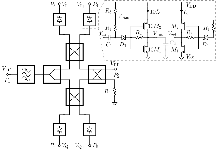
The six-port receiver performs complex down-conversion by additive mixing. The LO and RF inputs on ports \(P_1\) and \(P_2\) are superimposed in the linear, passive six-port core under four relative phases of \(0\), \(\pi/2\), \(\pi\) and \(3\pi/2\). The four resulting waveforms drive four power detectors, whose square-law nonlinearity produces two differential in-phase and quadrature pairs at the outputs \(P_3\) to \(P_6\). The baseband is recovered by subtraction,
\[ V_\mathrm{I} = V_\mathrm{I+} - V_\mathrm{I-}, \qquad V_\mathrm{Q} = V_\mathrm{Q+} - V_\mathrm{Q-}, \tag{1}\]
apart from a calibration of the static imbalances of the network (Mailand 2018). With \(f_\mathrm{RF} = f_\mathrm{LO}\) the receiver converts directly to baseband (homodyne). With an LO offset the same network becomes a heterodyne receiver with a low intermediate frequency (IF) (Hentschel 2005). The simulations in this documentation use the latter, with the LO at 159 GHz and the RF at 161 GHz, which gives a 2 GHz IF.
| Port | Signal | Function |
|---|---|---|
| \(P_1\) | \(V_\mathrm{LO}\) | LO input, through the BPF and the WPD to the two output couplers |
| \(P_2\) | \(V_\mathrm{RF}\) | RF input, through the RF coupler to the two output couplers |
| \(P_3\), \(P_4\) | \(V_\mathrm{I-}\), \(V_\mathrm{I+}\) | detector outputs of the in-phase pair |
| \(P_5\), \(P_6\) | \(V_\mathrm{Q+}\), \(V_\mathrm{Q-}\) | detector outputs of the quadrature pair |
| (core port 7) | fourth port of the RF coupler, terminated on chip by \(R_4 = 52\ \Omega\) |
Recommended reading on six-port receivers: the survey (Koelpin et al. 2010), the theory of the six-port as a communications receiver (Hentschel 2005), and the system analysis of its impairments and their calibration (Mailand 2018).
3 Getting Started
3.1 Requirements
Everything runs inside the IIC-OSIC-TOOLS container (Pretl and Zachl 2023; Fath et al. 2024), which ships the IHP Open-PDK (Herman et al. 2024), Xschem, ngspice, VACASK, KLayout, Magic, Netgen, kpex, GDSFactory, gds2palace, AWS Palace and snp2le. The repository follows the structure of the ihp-sg13g2-ams-chip-template, whose tutorial explains the folder layout and the Makefile conventions. SPARX extends it with the GDSFactory layout generator, the Palace EM flow, snp2le and the large-signal RF testbenches.
| Component | Version | Needed for |
|---|---|---|
| IIC-OSIC-TOOLS | 2026.10 or later |
every target |
| PDK | ihp-sg13g2 (set by .designinit, or sak-pdk ihp-sg13g2) |
every target except help and clean |
| IHP-GDSFactory-Addon | cloned and installed into .venv/ by make build-pdk |
layout generation and EM targets |
| VACASK | 1b48553 (2026-09-29) or later |
the PSS bench of the detector and the NF benches of the detector and the receiver, which run pss, pac and pnoise |
| snp2le | 0.1.10 or later | LE_NOISE=thermal, used by make sparx-core for the full-core fit |
The 2026.10 image ships VACASK fb8cc20 and snp2le 0.1.17. The images up to 2026.09 ship older VACASK builds: 2026.09 has hbnoise but neither pac nor pnoise, and 2026.08 has none of the three. On such a binary the shooting analyses of the PSS bench abort, the NF benches report pac and pnoise as unknown analyses and run the rest, and VACASK still exits 0. To check a binary:
strings $(which vacask) | grep -c "PNOISE periodic" # 0 on a build without pnoiseThe committed results were produced with a 1b48553 build, made inside the 2026.09 container as the testbench README describes. The Code-a-Chip notebook runs the fb8cc20 build of the 2026.10 image, see Section 15.
The Makefile checks $PDK when it is parsed. Every target except help and clean aborts if it is not ihp-sg13g2, because a wrong PDK mixes technologies silently: DRC and LVS would run against the wrong rule deck, and an extraction under ihp-sg13cmos5l exits cleanly with Metal5, TopMetal2, the MIM capacitors and both diodes missing from the netlist.
sak-pdk ihp-sg13g2 # switch the PDK of the running shell3.2 Quick Start
git clone https://github.com/iic-jku/SG13CMOS_SPARX.git
cd SG13CMOS_SPARX

make help                                       # every target
make build-top                                  # add-on, 160 GHz layout, render
make build-layout FREQ=77 NO_FILL=1             # 77 GHz, no metal fill
make klayout-verify CELL=sparx_powdet_sbd       # DRC, LVS, PEX of the detector
make sim-xschem TB=sparx_wpd_le_tb_acsp_vacask  # one testbench
make regression                                 # tool and flow smoke test
make all                                        # the complete flow
make all runs the Palace EM solves of the three blocks (Section 8.4) and 21 of the 24 testbenches, all except the three passive-model transients, several hours in total. The seven-port EM solve of the full core takes about 20 times the core-hours of the three blocks and runs only with make sparx-core or make all WITH_CORE=1. make help lists every target, and the repository README documents each of them with its parameters.
Most build outputs are committed: layouts, netlists, Palace results, Touchstone files, DRC and LVS reports, renders and simulation data. The targets overwrite them, and make clean deletes them, layout/ included. Check git status after a run and git restore what you did not mean to change. make release defaults to VERSION=2.0.0 and overwrites the committed release, so always pass a new VERSION.
3.3 Repository Structure
| Path | Contents |
|---|---|
Makefile, README.md |
the single flow for the whole chip, and the documentation of every target |
scripts/ |
six_port_gen.py (the layout generator), powdet_variant.py (detector variants), prune_pex_symbol.py, check_pex_ports.py, img2lay.py, logo assets/ |
layout/ |
generated GDS: sparx<FREQ>_top.gds for 60 GHz to 300 GHz, and the detector sparx_powdet_sbd.gds |
schematic/xschem/ |
detector, six-port and top-level schematics, and the symbols of the LE models |
testbenches/xschem/ |
24 ngspice and VACASK testbenches, the plot_simulations/ scripts with their data/ and figures/ |
netlist/ |
schematic/, layout/ and pex/ netlists of the detector, spice/ and spectre/ LE models from snp2le |
verification/drc/, verification/lvs/ |
DRC and LVS run folders |
verification/em/ |
layout/ (EM structures), metal_model/ (surface versus volume metal, Section 8.3), palace_model/ (Palace runs), s-parameter/ (Touchstone files), scripts/, stackups/ |
render/, release/, doc/ |
layout renders, published releases, this documentation |
sscs-ose-code-a-chip/ |
the Code-a-Chip notebook, see Section 15 |
measurements/ |
lab measurement notes |
Every folder with schematics has its own xschemrc, and the Makefile targets pass it with --rcfile. Netlists and simulator output of both folders land in testbenches/xschem/simulations/, so the relative includes of the testbenches always resolve. make open opens all design files in the sak-open.py file browser of the container.
4 Design Flow
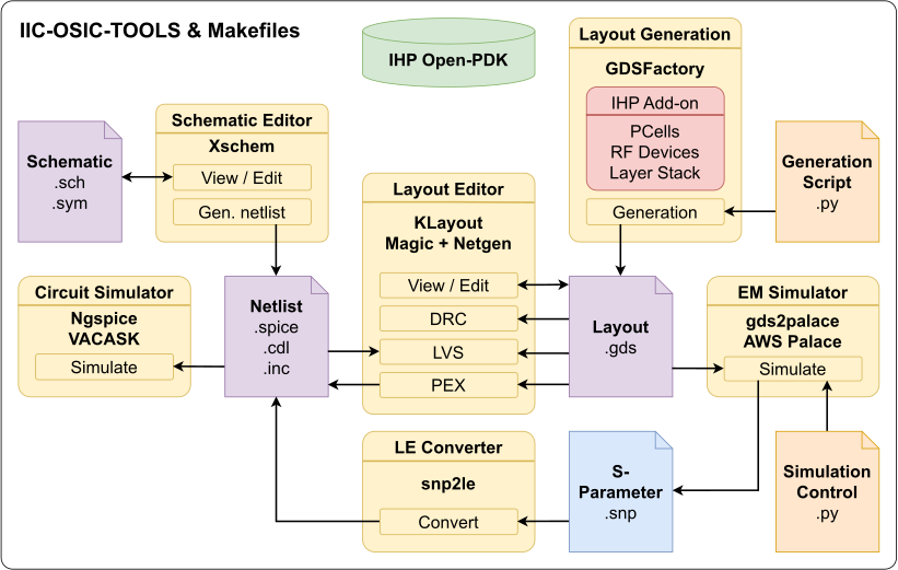
Figure 2 shows the flow. Schematics are entered in Xschem and simulated with ngspice and VACASK (Bűrmen 2026). The layout comes from a Python generation script on GDSFactory (Matres and GDSFactory Contributors 2023) with the IHP add-on (Kellerer-Pirklbauer and Dorrer 2026). KLayout and Magic with Netgen check it with DRC, LVS and PEX, and the extracted netlist goes back into simulation. gds2palace (Mühlhaus 2025) turns the EM structures of the same layout into AWS Palace (AWS Labs 2026) models, and snp2le (Dorrer 2026) turns the resulting S-parameters into SPICE and Spectre netlists that the circuit simulators read. The PDK is global to the flow and drawn without arrows: Xschem and the simulators read its symbols and models, KLayout and Magic its rule decks, gds2palace its layer stack, and the add-on wraps its PCells.
Nothing in the flow is specific to a six-port. The structure parameters live in one Python file, every step is a Makefile target, and every result is a file in the repository. This also lets an LLM agent drive the flow: it changes a parameter, rebuilds, and reads back the DRC, LVS and S-parameter results, while the designer sets the specification, reviews and signs off.
| Step | Tools | Make target | Output |
|---|---|---|---|
| Add-on install | git, pip | build-pdk |
IHP/, .venv/ |
| Layout generation | GDSFactory, IHP add-on | build-layout, build-layout-sweep |
layout/, verification/em/layout/ |
| Render | sak-render.py |
render-gds |
render/img/ |
| DRC | KLayout, Magic | klayout-drc, klayout-drc-regular, magic-drc |
verification/drc/ |
| LVS | Xschem, KLayout, Magic, Netgen | klayout-lvs, magic-lvs |
verification/lvs/, netlist/schematic/, netlist/layout/ |
| PEX | kpex, Magic | klayout-pex, magic-pex |
netlist/pex/ |
| EM simulation | gds2palace, AWS Palace | sim-bpf-em, sim-wpd-em, sim-blc-em, sim-sparx-core-em |
palace_model/ in verification/em/ |
| S-parameter copy | copy-sparam |
verification/em/s-parameter/ |
|
| LE models | snp2le | snp2le |
netlist/spice/, netlist/spectre/ |
| Circuit simulation | Xschem, ngspice, VACASK | sim-xschem, sim-all, sim-powdet-variants |
plot_simulations/ in testbenches/xschem/ |
| Full-core EM flow | AWS Palace, snp2le, ngspice, VACASK | sparx-core |
core EM, both fits, two benches |
| Everything | all of the above, the full-core EM flow only with WITH_CORE=1 |
all |
|
| Smoke test | a subset of the above | regression, regression-full |

make all runs in five stages. Each header names the folders its stage writes to, and the targets of a stage run from top to bottom. An indented target is called by the nearest target above it with less indent, a box marked ×N stands for N calls of the same target, and the second line of a box shows the parameters of the call. The dashed boxes run only with WITH_CORE=1, and the LVS of the top cell is not part of make all yet.
Figure 3 shows how the targets of Table 6 are chained. All of them live in the one top-level Makefile, and every arrow is a direct $(MAKE) call. make all runs the stages from left to right, so the testbenches simulate the LE models that the same run has just fitted. The two dashed boxes are the EM solve and the fit of the full core. make all runs them only with WITH_CORE=1, through make sparx-core after the block fits. That step also runs the two sparx_core_tb_acsp_* benches, which sim-all repeats. With the default WITH_CORE=0, make all simulates the committed full-core fit in the sparx_core_le_tb_acsp_* and sparx_top_le_tb_* benches. After a change to a structure parameter in scripts/six_port_gen.py, run make sparx-core or make all WITH_CORE=1, or those benches keep showing the core of the old layout. The top cell is drawn as sparx*_top because it follows the design frequency: make all checks sparx160_top, and make all FREQ=<GHz> the top cell of that frequency (Section 5.5). The LVS box of the top cell is drawn ahead of the flow: make all runs it once top-level LVS works (Section 14). The figure leaves out the helper steps: copy-sparam after the EM runs, the schematic netlist export inside klayout-lvs and magic-lvs, and the symbol-pex call inside the two PEX targets.
5 Programmatic Layout Generation
5.1 The GDSFactory IHP Add-On
SPARX is built on the IHP-GDSFactory-Addon (Kellerer-Pirklbauer and Dorrer 2026), a GDSFactory integration of the IHP Open-PDK developed for this project. It wraps the foundry PCells and the technology layer stack for use from Python and adds a library of RF devices: transmission lines and corners, the branch-line coupler, the Wilkinson power divider, coupled-line and hairpin coupled-line bandpass filters, a directional coupler and a quarter-wave transformer. Because the add-on wraps the foundry PCells instead of copying them, a layout change inside a PDK cell needs no wrapper update. Only a change of a cell’s interface has to be followed.
make build-pdk clones the add-on into IHP/ and installs it into .venv/, and the layout and EM targets run in that environment.
5.2 The Generator
scripts/six_port_gen.py takes the design frequency as its only design input and builds the complete chip:
- effective permittivity and guided wavelength from the closed-form models of Section 5.3,
- three BLCs, one WPD and one hairpin BPF, assembled into the six-port core with its interconnects,
- four SBD power detectors with their MIM decoupling, fed from the core outputs through dedicated via stacks,
- the 52 \(\Omega\) termination of the RF coupler, the probe pads, the bond pads, the seal ring, logos and author labels,
- TopMetal2 and Metal5 fill,
- the top-level GDS, the detector GDS, and the EM sub-structures with their Palace port markers.
make build-layout                       # layout/sparx160_top.gds
make build-layout FREQ=77               # layout/sparx77_top.gds
make build-layout FREQ=77 NO_FILL=1     # no metal fill, fast preview
make build-layout FREQ=77 NO_FILL_M5=1  # no Metal5 ground fill only
build-layout also writes the EM sub-structures to verification/em/layout/: the BLC, the WPD, the BPF and the bare six-port core, each with one Palace port marker layer per port, from layer 201 up to layer 207 for the seven-port core. The EM targets solve exactly these files, so the EM results always describe the structures that are instantiated in the chip.
Every structure parameter lives in the generator. Change it there, rerun build-layout, then rerun the EM target.
Parameter in six_port_gen.py |
Value | Meaning |
|---|---|---|
--frequency |
160e9 |
design frequency in Hz, set by make build-layout FREQ=<GHz> |
e_r |
4.1 |
relative permittivity of the back-end oxide |
Z0 |
50 |
reference impedance in \(\Omega\) |
signal_cross_section |
topmetal2_routing |
signal layer of every line |
ground_cross_section |
metal5_routing |
ground plane under every line |
order |
3 |
BPF order |
filter_type |
butter |
BPF prototype, butter (Butterworth) or cheby (Chebyshev) |
ripple_dB |
3 |
passband ripple of the Chebyshev prototype, ignored for Butterworth |
bandwidth |
1e9 |
absolute bandwidth in Hz handed to the BPF synthesis |
wpd_shape |
U |
routing shape of the WPD, C or U |
The EM port settings SIGNAL_CROSS_SECTION, GROUND_CROSS_SECTION and Z0 of the Makefile are passed to the Palace driver and are not read from the layout, so they must match signal_cross_section, ground_cross_section and Z0 here.
5.3 Closed-Form Analytical Models
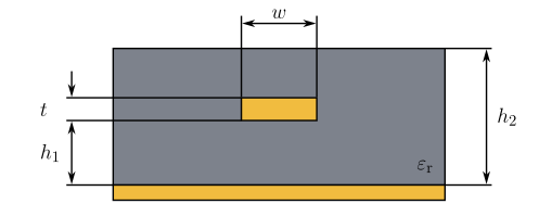
Every passive is built from embedded microstrip lines, defined by their width \(w\) and length \(l\) and by the metal layers they use. Figure 4 shows the cross-section: \(t\) is the conductor thickness, \(h_1\) the distance from the conductor to the ground plane, and \(h_2\) the total dielectric height including the oxide above the conductor. The width sets the characteristic impedance \(Z_0\), and the length scales with the guided wavelength \(\lambda_\mathrm{g} = \lambda_0 / \sqrt{\varepsilon_\mathrm{r,eff}}\), with \(\lambda_0\) the free-space wavelength.
The generator combines two IPC-2141 closed-form expressions (IPC 2004), chosen by comparison with EM simulation. \(Z_0\) comes from the surface-microstrip formula, which matches the EM results more closely than the embedded-microstrip impedance formula,
\[ Z_0 = \frac{87.0\ \Omega}{\sqrt{\varepsilon_\mathrm{r} + 1.41}}\,\ln\!\left(\frac{5.98\,h_1}{0.8\,w + t}\right), \tag{2}\]
and \(\varepsilon_\mathrm{r,eff}\) from the embedded-microstrip approximation, which accounts for the oxide above the conductor through the ratio \(h_2/h_1\),
\[ \varepsilon_\mathrm{r,eff} = \varepsilon_\mathrm{r}\left[1 - \exp\!\left(-1.55\,\frac{h_2}{h_1}\right)\right]. \tag{3}\]
Table 8 lists the geometry of six signal and ground combinations of the seven-layer SG13G2 metal stack (Herman et al. 2024), where \(z_\mathrm{sig}\) is the height of the lower conductor edge and \(z_\mathrm{gnd}\) that of the upper ground edge, so \(h_1 = z_\mathrm{sig} - z_\mathrm{gnd}\). SPARX uses TM2 over M5: \(t = 3\ \mu\)m, \(h_1 = 5.65\ \mu\)m, \(h_2 = 10.15\ \mu\)m and \(\varepsilon_\mathrm{r} = 4.1\).
| Combination | \(z_\mathrm{sig}\) (\(\mu\)m) | \(z_\mathrm{gnd}\) (\(\mu\)m) | \(h_1\) (\(\mu\)m) | \(h_2\) (\(\mu\)m) | \(t\) (\(\mu\)m) |
|---|---|---|---|---|---|
| TM2 over M1 | 11.23 | 1.46 | 9.77 | 14.27 | 3.0 |
| TM2 over M5 | 11.23 | 5.58 | 5.65 | 10.15 | 3.0 |
| TM2 over TM1 | 11.23 | 8.43 | 2.80 | 7.30 | 3.0 |
| TM1 over M1 | 6.43 | 1.46 | 4.97 | 14.27 | 2.0 |
| TM1 over M2 | 6.43 | 2.49 | 3.94 | 13.24 | 2.0 |
| TM1 over M5 | 6.43 | 5.58 | 0.85 | 10.15 | 2.0 |
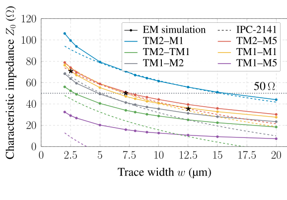
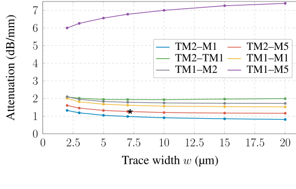
Figure 5 confirms the range \(0.1 \le w/h_1 \le 2\) that IPC-2141 states for Equation 2, for every combination with \(h_1 > t\). For TM2 over M5, Equation 2 gives 2.5 \(\mu\)m, 7.2 \(\mu\)m and 12.5 \(\mu\)m for the \(\sqrt{2} Z_0 = 70.7\ \Omega\), \(Z_0 = 50\ \Omega\) and \(Z_0/\sqrt{2} = 35.4\ \Omega\) the WPD and the BLCs need (Wilkinson 1960; Reed and Wheeler 1956). At these widths the EM simulation gives 74.1 \(\Omega\), 51.1 \(\Omega\) and 39.4 \(\Omega\), which is 4.7 %, 2.2 % and 11.5 % above target, the last beyond \(w/h_1 = 2\). Where \(h_1 < t\) the closed form is off by more than 14 % at every width and is of no use.
The TM1 rows estimate what IHP’s five-layer SG13CMOS5L stack would allow, with one thick top metal and four thin layers. By Figure 5 and Figure 6 the only usable combination there is TM1 over M2, which corresponds to TM1 over M1 in SG13CMOS5L.
The widths of the WPD and the BLCs follow from their impedances through Equation 2, and their quarter-wave lengths \(\lambda_\mathrm{g}/4\) through Equation 3. The hairpin BPF is synthesized from a Butterworth or Chebyshev prototype (Cristal and Frankel 1972; Hong and Lancaster 2001). Since every computation is closed-form, all widths and lengths follow directly from the design frequency, without optimization loops, iterations or training data.
5.4 Design Considerations
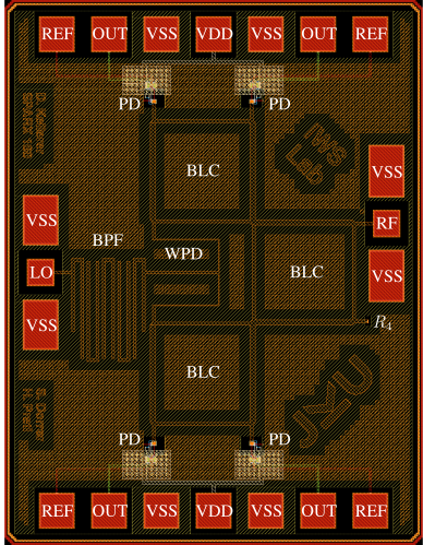
- Pads. The top and bottom rows are bond pads for PCB bonding, each row with
REF,OUT,VSS,VDD,VSS,OUT,REFfor two detectors. The left and right rows are ground-signal-ground probe pads for the LO and the RF input, for wafer probing. - WPD without isolation resistor. A standard WPD carries an isolation resistor that dissipates the imbalance between its outputs. Under the matched, in-phase, equal-amplitude condition of the forward-dividing path of the six-port, the resistor can be omitted (Wilkinson 1960). At mm-wave frequencies the omission is also a physical necessity: a 100 \(\Omega\) resistor with its connections exceeds the \(\lambda_0/10\) rule of thumb for lumped elements. The price is the limited output isolation of a resistor-less divider, acceptable because both outputs see symmetric, matched loads.
- Placement. The three BLCs sit corner to corner to minimize conductor loss and phase mismatch. The WPD is mirrored into the otherwise empty center of the core, which saves area and shortens the path to the BLC inputs.
- Termination. The 52 \(\Omega\) silicided poly resistor \(R_4\) broadband-matches the fourth port of the RF coupler. It connects to TM2 through a via stack, with Metal5 no-fill regions around it to reduce the parasitic capacitance.
- Detector feed. A dedicated via stack routes each BLC output through the MIM coupling capacitor \(C_1\) straight to the SBD of its detector, to keep interconnect loss and parasitics low.
5.5 Frequency Scaling
make build-layout-sweep            # 60 GHz to 300 GHz in 20 GHz steps
make build-layout-sweep START_FREQ=60 STOP_FREQ=300 STEP_FREQ=20 NO_FILL=1
The sweep builds the thirteen layouts in layout/ in under one minute. The core scales with the wavelength, while the pad frame and the detectors do not, so from about 220 GHz up the pad frame sets the die width:
layout/, in \(\mu\)m.
| Frequency | 60 GHz | 100 GHz | 160 GHz | 200 GHz | 300 GHz |
|---|---|---|---|---|---|
| Die outline | 1926 × 2523 | 1409 × 1759 | 1118 × 1329 | 1021 × 1186 | 1010 × 994 |
All thirteen layouts pass the KLayout DRC at macro level, and their EM simulations are clean as well. The repository commits the DRC reports, the EM results and the fitted models of 160 GHz only. Any other frequency reruns the same targets with FREQ=<GHz>, for example make build-layout FREQ=80, make klayout-drc FREQ=80 and make sim-bpf-em FREQ=80.
5.6 Renders
make render-gds renders the top-level GDS with sak-render.py into render/img/: all mask layers on a white and on a black background, and a TopMetal2-only view that shows the RF structures without the ground plane underneath.
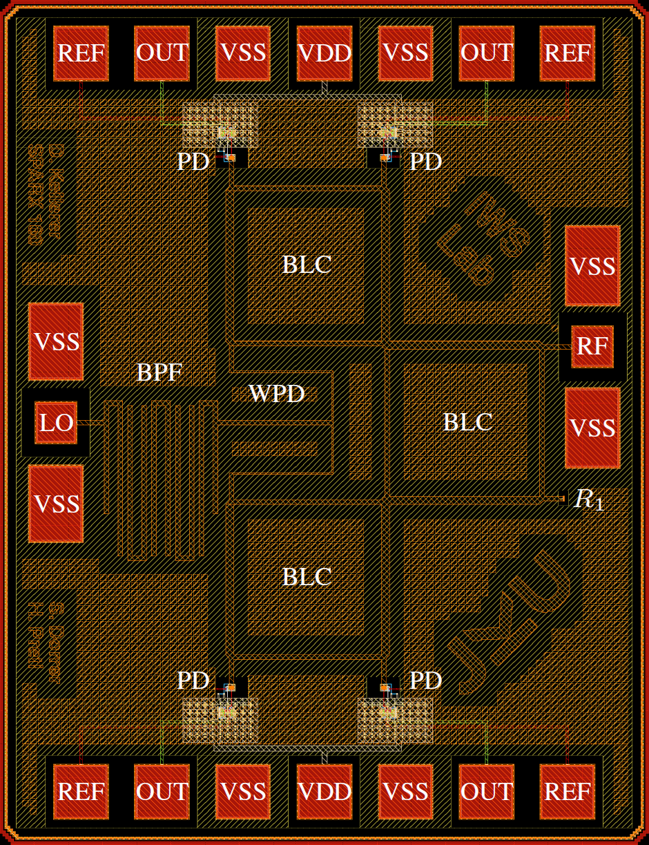
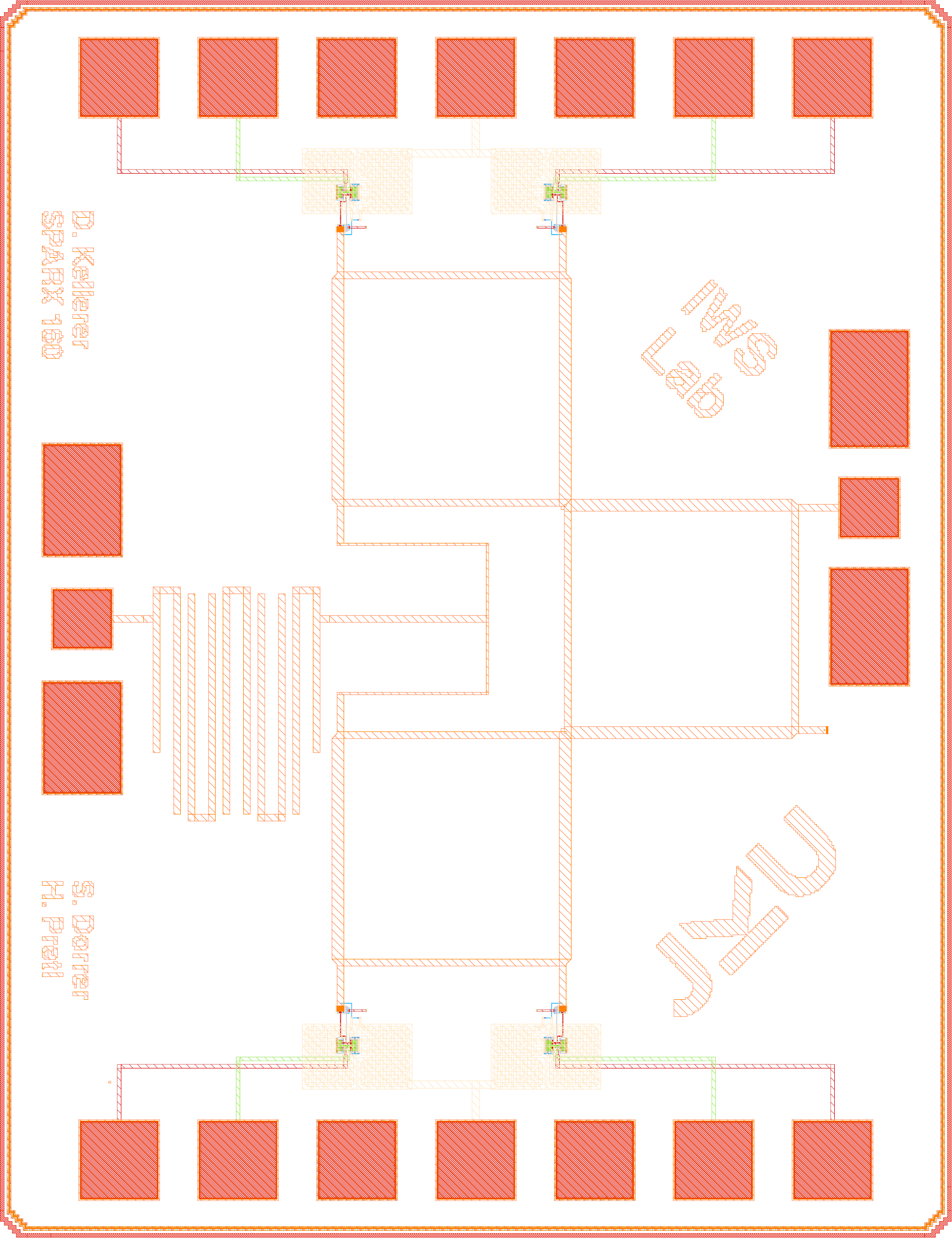
The renders above are of the taped-out GDS, release/v.1.0.0/gds/RFFE6027.gds. The generator has evolved since the tapeout, so the current layout/sparx160_top.gds differs in outline and in placement details from the fabricated die in Figure 17. Use the release GDS for anything that has to match the silicon.
6 SBD Power Detector
6.1 Circuit
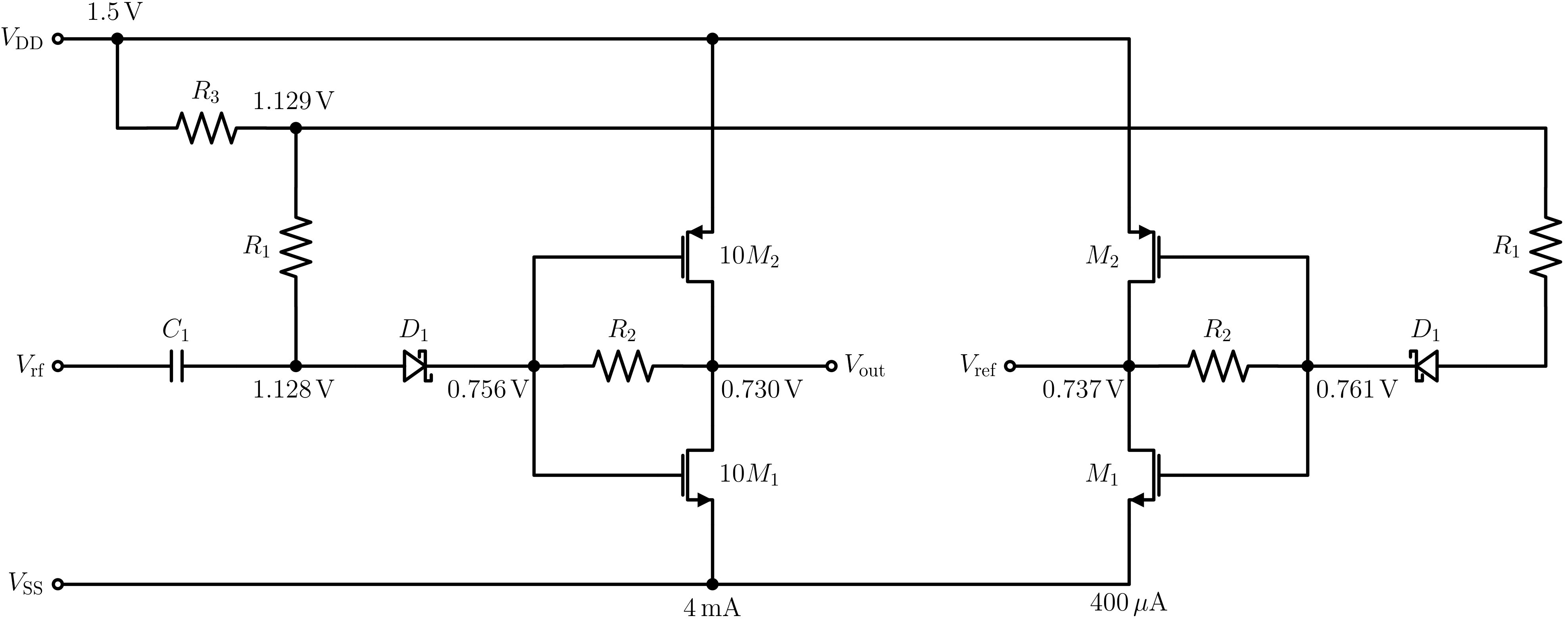
The detector input \(V_\mathrm{in}\) from a BLC output is ac-coupled through \(C_1\) to a forward-biased Schottky diode \(D_1\) and broadband-terminated by the silicided poly resistor \(R_1\). The diode current drives a TIA, a CMOS inverter of \(M_1\) and \(M_2\) with the feedback resistor \(R_2\), which delivers a buffered output \(V_\mathrm{out}\). A replica branch with its own diode and TIA produces \(V_\mathrm{ref}\), so the output is read differentially as \(V_\mathrm{out} - V_\mathrm{ref}\). That removes the dc offset, rejects common-mode noise and tracks thermal drift (Jonsson et al. 2014). \(M_1\) and \(M_2\) have minimum length and run in strong inversion (\(g_\mathrm{m}/I_\mathrm{D} \approx 6\) S/A) for bandwidth. The detector branch uses ten of each in parallel and draws 4 mA, the replica one of each and 400 \(\mu\)A. The low-pass capacitor \(C_2\) is off chip, which saves area and leaves the cutoff to the measurement setup. Schottky diodes in foundry CMOS have been used for mm-wave detection before (Sankaran and O 2005; Han et al. 2011).
| Symbol | Type | Value |
|---|---|---|
| \(V_\mathrm{DD}\) | supply | 1.50 V |
| \(V_\mathrm{bias}\) | operating point | 1.13 V |
| \(V_\mathrm{ref}\) | operating point | 0.74 V |
| \(I_\mathrm{q}\) | replica current | 400 \(\mu\)A |
| \(R_1\), and \(R_4\) of the core | silicided poly | 52 \(\Omega\) |
| \(R_2\) | poly | 911 \(\Omega\) |
| \(R_3\) | high-resistance poly | 6.23 k\(\Omega\) |
| \(C_1\) | MIM | 150 fF |
| \(C_2\) | off chip | 5 pF |
| \(M_1\) | NMOS | \(W/L\) = 5 \(\mu\)m / 0.13 \(\mu\)m, ten in parallel in the detector branch |
| \(M_2\) | PMOS | \(W/L\) = 10 \(\mu\)m / 0.13 \(\mu\)m, ten in parallel in the detector branch |
| \(D_1\) | SBD (schottky_nbl1) |
\(m = 1\) unit cell as fabricated, \(m = 16\) in the revised design |
6.2 Three Versions
The detector is characterized in three versions, all at the typical corner and 27 °C from a 50 \(\Omega\) source. There is one schematic, and scripts/powdet_variant.py rewrites the emitted netlist before the simulator sees it:
VARIANT |
Version | What the rewrite does |
|---|---|---|
| (none) | \(m = 1\), fabricated | nothing, the schematic as taped out |
m1_pex |
post-layout | the schematic subcircuit replaced by the Magic full-RC extraction from netlist/pex/ |
m16 |
revised | both Schottky instances set to 16 parallel unit cells |
make sim-xschem TB=sparx_powdet_sbd_tb_pss_vacask VARIANT=m16
make sim-powdet-variants        # PSS and NF benches for m16 and m1_pex
At tapeout in March 2026 the detector was checked with a two-tone HB sweep in VACASK. It confirmed square-law detection, \(V_\mathrm{IF} \propto V_\mathrm{RF} V_\mathrm{LO}\), but says nothing about the absolute responsivity, the match, the compression or the noise. The TN, HBAC, HBNOISE, shooting PSS, PAC and PNOISE analyses that VACASK gained later in 2026 characterize the detector as a receiver front-end.
6.3 Transfer Curve, Responsivity and Input Impedance
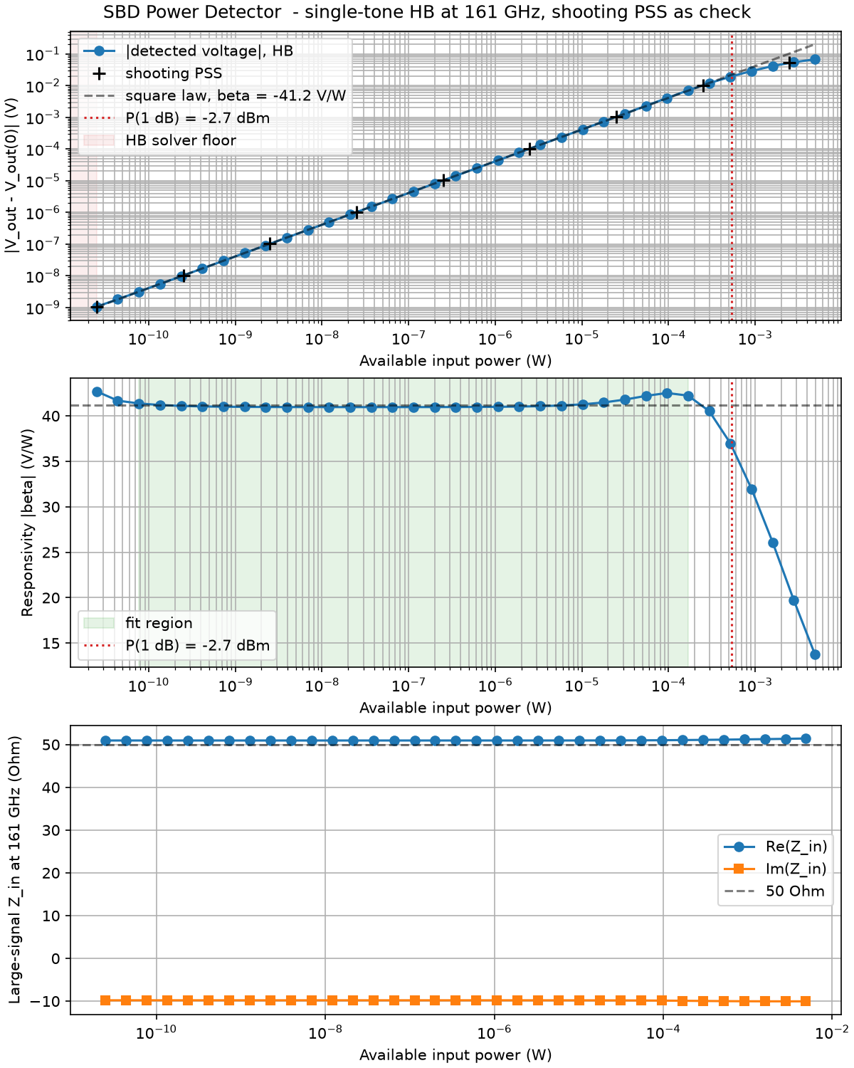
sparx_powdet_sbd_tb_pss_vacask).
The responsivity \(\beta = \Delta V_\mathrm{out} / P_\mathrm{in}\) is the detected output voltage per available input power, with \(\Delta V_\mathrm{out}\) the differential output measured from its zero-drive value. The coupling efficiency \(\eta = (\beta / R_2) / \beta_{I,\mathrm{max}}\) compares the rectified current with that of an ideal square-law junction, \(\beta_{I,\mathrm{max}} = 1/(2 n V_\mathrm{T}) = 18.29\) A/W for an ideality factor \(n = 1.057\) and \(V_\mathrm{T} = 25.86\) mV (Cowley and Sorensen 1966; Han et al. 2011).
| Quantity | \(m = 1\), fabricated | \(m = 1\), post-layout | \(m = 16\) |
|---|---|---|---|
| Responsivity \(\beta\) | 41.2 V/W | 38.8 V/W | 250.8 V/W |
| 1 dB compression | -2.7 dBm | -2.4 dBm | -13.3 dBm |
| Input impedance at 161 GHz | (51 - j10) \(\Omega\) | (40 - j25) \(\Omega\) | (28 - j28) \(\Omega\) |
| Coupling efficiency \(\eta\) | 0.25 % | 0.23 % | 1.5 % |
| Video bandwidth | 1.24 GHz | 1.08 GHz | 1.60 GHz |
The responsivity of the fabricated detector is flat from -71 dBm to -8 dBm, and its input impedance stays at \((51 - \mathrm{j}10)\ \Omega\) up to compression. HB and shooting PSS agree within 0.6 % from -66 dBm to +4 dBm. The two algorithms share no code, so the agreement is an independent check of the curve.
The coupling efficiency is what limits the detector. The PDK Schottky unit cell has a series resistance of 1.36 k\(\Omega\) against a junction resistance of 0.9 k\(\Omega\) at its 30 \(\mu\)A bias, so the 52 \(\Omega\) termination that gives the flat, drive-independent match passes only about 2 % of the input power into the diode branch, and the series resistance and the junction capacitance take most of that at 161 GHz. Sixteen parallel cells cut the series resistance 16-fold and raise \(\beta\) to 251 V/W, at the cost of a worse match and an earlier compression. PEX lowers \(\beta\) by 6 % and the video bandwidth by 13 %.
6.4 Noise, NEP and Noise Figure
The noise-equivalent power, the input power that gives a signal-to-noise ratio of one in a 1 Hz bandwidth, is
\[ \mathrm{NEP}(f) = \frac{\sqrt{S_v(f)}}{\beta\,\lvert H(f) \rvert}, \tag{4}\]
with \(S_v(f)\) the output noise density and \(\lvert H(f) \rvert\) the normalized video response from HBAC (Han et al. 2011). For the fabricated detector it falls from 8.7 nW/\(\sqrt{\text{Hz}}\) at 1 MHz to 226 pW/\(\sqrt{\text{Hz}}\) at 1 GHz, and 97 % of the output noise power is flicker noise of the parasitic vertical PNP inside the PDK model of the Schottky diode, so nothing that was sized in this design sets the noise floor. Detecting at dc, as a conventional six-port does, pays for that flicker noise: an LO offset to a 1 GHz IF improves the NEP 38-fold. The 16-cell design reaches 13.5 pW/\(\sqrt{\text{Hz}}\) at 1 GHz.
In the LO-offset mode the detector is a mixer, and its double-sideband noise figure follows from the conversion gain \(g = \lvert V_\mathrm{IF} \rvert^2 / (2 P_\mathrm{RF})\) of the upper and lower sideband from HBAC and the output noise density under LO drive from HBNOISE,
\[ F_\mathrm{DSB} = 1 + \frac{S_v(f_\mathrm{IF})}{(g_\mathrm{U} + g_\mathrm{L})\, k T_0}, \tag{5}\]
with \(k\) the Boltzmann constant and \(T_0 = 290\) K. The double-sideband definition applies to homodyne operation (Razavi 2012), and the low-IF mode adds 3 dB.
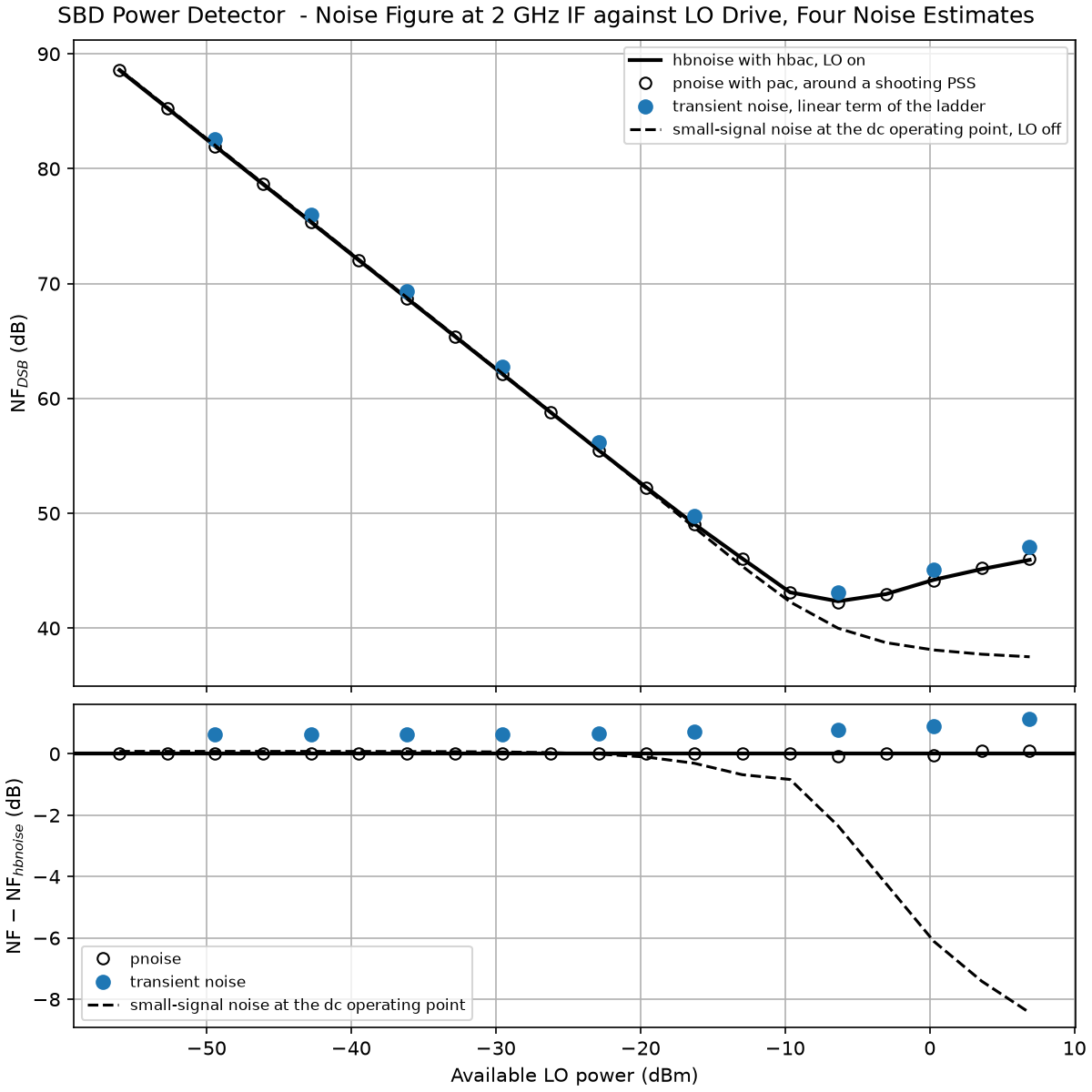
sparx_powdet_sbd_tb_tn_lo_vacask).
| Quantity | \(m = 1\), fabricated | \(m = 1\), post-layout | \(m = 16\) |
|---|---|---|---|
| NEP at 1 MHz | 8.7 nW/\(\sqrt{\text{Hz}}\) | 9.5 nW/\(\sqrt{\text{Hz}}\) | 0.72 nW/\(\sqrt{\text{Hz}}\) |
| NEP at 1 GHz | 226 pW/\(\sqrt{\text{Hz}}\) | 247 pW/\(\sqrt{\text{Hz}}\) | 13.5 pW/\(\sqrt{\text{Hz}}\) |
| Minimum \(\mathrm{NF}_\mathrm{DSB}\) at 2 GHz IF, HBNOISE | 42.3 dB at -6.3 dBm | 42.7 dB at -6.3 dBm | 26.8 dB at -3.0 dBm |
| Minimum detectable power, 1 MHz to 5 GHz | -16.6 dBm | -16.2 dBm | -27.3 dBm |
Figure 12 compares the four noise estimates. PAC and PNOISE reproduce HBAC and HBNOISE within 0.2 dB, and the transient noise, which needs no linearization, lies 0.6 dB to 1.1 dB above them. The conventional small-signal noise at the dc operating point is 2.3 dB optimistic at the minimum and 8.4 dB at +6.9 dBm, where it predicts a falling noise figure that every large-signal analysis shows rising. A mixer noise figure therefore needs a large-signal noise analysis.
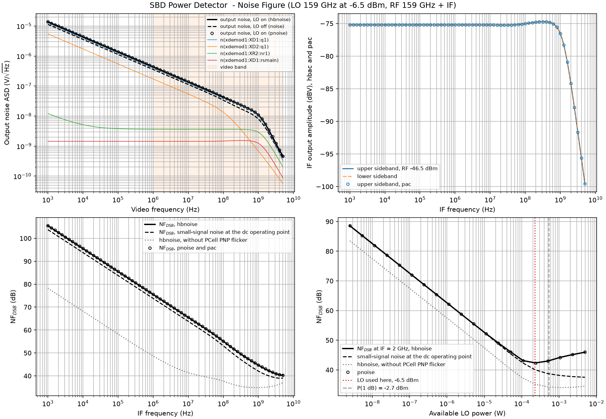
sparx_powdet_sbd_tb_nf_vacask).
The dominant noise source is a model extrapolation: the PNP flicker model is evaluated at about 20 pA of base current, far below any plausible characterization current, so the scripts also report every figure with those contributors removed. Measurements will show which of the two applies. The VACASK builds since 2026-09-07 also scale the base-collector saturation current of that PNP with its area once instead of twice, which raises the noise power of every PNP-dominated quantity 1.95-fold compared with ngspice and the VACASK of the 2026.08 image.
Every number of this section is traced to its testbench, data file and field, with all equations derived, in testbenches/xschem/SBD-PD-RESULTS.md. The testbench README describes the benches, their settings and their limits.
7 Physical Verification
7.1 DRC
Both flows use sak-drc.sh and write per-cell run folders, verification/drc/<CELL>.klayout.drc/ with a .lyrdb report and verification/drc/<CELL>.magic.drc/. DRC_LEVEL selects the KLayout rule set, while Magic always runs the full rule set of its tech file.
sak-drc.sh sets them.
| Check | precheck |
macro (default) |
regular |
|---|---|---|---|
| Foundry precheck rule set | \(\checkmark\) | \(\checkmark\) | \(\checkmark\) |
| Pin and label checks | \(\checkmark\) | \(\checkmark\) | \(\checkmark\) |
| Full FEOL and BEOL rules, off-grid, angle, recommended rules | \(\checkmark\) | \(\checkmark\) | |
| Density, extra rules, antenna | \(\checkmark\) |
make klayout-drc                                        # top cell, DRC_LEVEL=macro
make klayout-drc-regular                                # top cell, full rule set
make klayout-drc CELL=sparx_powdet_sbd DRC_LEVEL=regular
make magic-drc CELL=sparx_powdet_sbd
The 160 GHz top cell has no violations at macro level, and neither have the generated layouts of the other twelve frequencies. At regular level the 160 GHz top cell shows 33 antenna violations, which IHP waived for the March 2026 tapeout:
regular level, waived for the tapeout.
| Rules | Count | Cause |
|---|---|---|
Ant.e_Metal5, Ant.e_TopMetal1, Ant.e_TopMetal2 |
24 | large RF and supply metal, the Metal5 ground plane on vss included, connects to the gates of the detector transistors and the dummy devices |
Ant.f_TopVia2 |
8 | the same nets, TopVia2 to gate area |
Ant.h |
1 | the antenna diode built into the schottky PCell sits in NWell, a quirk of the device cell |
7.2 LVS
LVS compares the GDS against a netlist exported from Xschem: CDL for KLayout (klayout-lvs) and SPICE for Magic with Netgen (magic-lvs). Both ignore the ntap and ptap substrate contacts. EV_PRECISION sets the significant digits of Xschem’s device-parameter evaluation, to avoid rounding mismatches between Xschem and KLayout.
make klayout-lvs CELL=sparx_powdet_sbd
make magic-lvs CELL=sparx_powdet_sbd
The power detector passes LVS in both flows. Top-level LVS is open, blocked by the Rmetal handling of the PDK (IHP-Open-PDK issue 1041).
7.3 PEX
make magic-pex CELL=sparx_powdet_sbd               # EXT_MODE=3, full RC
make klayout-pex CELL=sparx_powdet_sbd             # kpex with the Magic engine
EXT_MODE selects C-decoupled (1), C-coupled (2) or full-RC (3, the default) extraction. kpex has no C-decoupled mode and falls back to C-coupled for 1. The netlists land in netlist/pex/<CELL>_<tool>_pex_<EXT_MODE>.spice, so the modes do not overwrite each other. Both targets first rebuild the PEX symbol schematic/xschem/<CELL>_pex.sym from <CELL>.sym, reorder the subcircuit pins to match it, and finish with scripts/check_pex_ports.py, which fails the target if a declared port does not reach the circuit. Such a netlist simulates without a warning while the cell behaves differently.
For full-RC extraction magic-pex gates extresist by resistance, not by delay (THRESHOLD=1000, MINRES=100, MINDELAY=0, in m\(\Omega\) and ps). A delay gate of 1 ps is 58° at 160 GHz and drops the baseband route resistances that matter for the TIA.
The committed post-layout netlist netlist/pex/sparx_powdet_sbd_magic_pex_3.spice carries a correction: the full-RC run with this Magic version hits magic#557 and emits the coupling capacitance twice, so the capacitance per net pair was rebuilt from a reference extraction of the same layout, as its header documents. Rerunning make magic-pex overwrites that correction. Against the schematic, the extraction lowers the responsivity by 5.9 %, detunes the input impedance from \((51 - \mathrm{j}10)\ \Omega\) to \((40 - \mathrm{j}25)\ \Omega\) and lowers the video bandwidth by 13 %.
8 EM Simulation
8.1 Flow
The EM targets solve the structures build-layout wrote to verification/em/layout/. gds2palace (Mühlhaus 2025) builds the mesh and the configuration from the GDS and the port markers, and AWS Palace (AWS Labs 2026) runs a driven frequency-domain solve. The raw and the de-embedded Touchstone files land in verification/em/palace_model/<name>_data/output/<name>/, and copy-sparam copies both to verification/em/s-parameter/.
make build-layout && make sim-wpd-em     # likewise sim-blc-em, sim-bpf-em
make copy-sparam SPARAM=sparx160_wpd
make view-em-sim FILE_NAME=sparx160_wpd.s3p
make sparx-core # seven-port core: EM, copy, fit, benches| Setting | Value |
|---|---|
| Process stackup | SG13G2_nosub.xml from $PDK_ROOT/$PDK/libs.tech/palace/XML_stackup/legacy/ (workflow/ in older PDKs), not vendored |
| Ports | TopMetal2 signal over Metal5 ground, 50 \(\Omega\) (SIGNAL_CROSS_SECTION, GROUND_CROSS_SECTION, Z0) |
| Metal model | gds2palace’s surface model, a surface impedance on every metal face, see Section 8.3 |
| Frequency sweep | 80 GHz to 240 GHz in 1.6 GHz steps, 101 points, adaptive sweep tolerance 0.02 |
| Element order | 2 |
| Linear solver | GMRES, tolerance \(10^{-6}\) |
| MPI ranks | 12 for the committed block runs, 128 for the core, NP=4 by default |
The stackup leaves the substrate out: the solid Metal5 plane under the TopMetal2 lines shields the silicon, so the model loses almost nothing in accuracy and saves a large part of the mesh. verification/em/stackups/README.md describes the available stackups and the XML format.
On a host with fewer than four physical cores, Open MPI aborts with “not enough slots”. Lower NP, or set OMPI_MCA_hwloc_base_use_hwthreads_as_cpus=1 as the regression workflow does.
8.2 Results at 160 GHz
All structures are simulated as generated by the closed-form models, without any tuning. Table 17 gives the de-embedded results of the 160 GHz chip blocks from verification/em/s-parameter/. The snp2le models of Section 9 are fitted from the raw files instead.
| Block | Ports | Results at 160 GHz |
|---|---|---|
| BLC | 4 | \(\lvert S_{11} \rvert\) = -26.3 dB, through \(\lvert S_{21} \rvert\) = -4.7 dB, coupled \(\lvert S_{31} \rvert\) = -3.1 dB, isolation \(\lvert S_{41} \rvert\) = -16.2 dB, amplitude imbalance 1.6 dB, phase difference -86.6° |
| WPD | 3 | \(\lvert S_{11} \rvert\) = -19.0 dB, \(\lvert S_{21} \rvert\) = \(\lvert S_{31} \rvert\) = -4.4 dB, output imbalance below 0.01 dB and 0.1°, output isolation \(\lvert S_{23} \rvert\) = -7.9 dB |
| BPF | 2 | \(\lvert S_{11} \rvert\) = -6.2 dB, \(\lvert S_{21} \rvert\) = -10.0 dB, 3 dB passband from 150 GHz to 171 GHz |
The BLC splits within 1.6 dB and 3.4° of the ideal quadrature, which is acceptable for six-port operation (Laemmle et al. 2012, 2013). The resistor-less WPD isolates its outputs by 7.9 dB, close to the 6 dB of an ideal resistor-less divider. The hairpin BPF combines meanders and coupled lines, where the closed-form models reach their limits: its loss and match are the weakest results of the core, and it sits in the LO path. This motivates a hybrid strategy that keeps the closed form for the simple, frequency-scalable structures and spends EM-driven or AI-assisted optimization on the inherently complex ones.
The full core is solved as one seven-port structure including all interconnects and the via stack down to \(R_4\), without the probe pads. Table 18 lists what a six-port receiver depends on, the amplitude and phase imbalance between the two outputs of each output coupler:
| Pair | Amplitude imbalance | Phase difference |
|---|---|---|
| from the LO port, \(\lvert S_{41} \rvert - \lvert S_{31} \rvert\) | 1.9 dB | -82.9° |
| from the LO port, \(\lvert S_{51} \rvert - \lvert S_{61} \rvert\) | 1.3 dB | -82.4° |
| from the RF port, \(\lvert S_{32} \rvert - \lvert S_{42} \rvert\) | 3.0 dB | -85.3° |
| from the RF port, \(\lvert S_{62} \rvert - \lvert S_{52} \rvert\) | 0.8 dB | -102.5° |
The insertion loss at 160 GHz is 16.7 dB to 18.6 dB from the LO port to the four outputs and 6.5 dB to 10.7 dB from the RF port, into 50 \(\Omega\). The phase differences deviate from the ideal -90° by 5° to 12.5°. Imbalances of this size are static, and six-port calibration removes them (Mailand 2018). The losses come from the surface metal model and are slightly pessimistic, see Section 8.3.
8.3 Metal Model
gds2palace models a metal either as a hollow shell with a surface impedance on every face, its default and the model of all SPARX runs, or as a conducting volume whose current Palace solves inside the metal. A check of 2026-10-18 compared the surface results with a 2D volume reference of the TopMetal2-over-Metal5 line and with volume physics emulated on the blocks. The 2.5 \(\mu\)m WPD arms agree within 1 %, the 7.2 \(\mu\)m 50 \(\Omega\) lines read 6 % to 14 % too lossy from 80 GHz to 240 GHz, and the BPF passband would improve by about 0.5 dB. Three errors of the surface model partly cancel: Palace’s thickness correction treats the 0.49 \(\mu\)m Metal5 ground as carrying current on both faces and reads it too lossy, the 2 \(\mu\)m mesh reads 2 % to 6 % high, and the surface impedance reads narrow, thick strips low. A volume solve that resolves the 0.23 \(\mu\)m skin depth of TopMetal2 at 160 GHz needs several times the memory of the available hosts, and the error is conservative, so the flow stays on the surface model for now. verification/em/metal_model/README.md explains the two models, documents the check with its scripts and results, and lists when to switch to volume metal.
8.4 Cost
palace.json.
| Structure | Ports | Mesh elements | Unknowns | MPI ranks | Peak memory | Wall time |
|---|---|---|---|---|---|---|
| WPD | 3 | 34 927 | 243 286 | 12 | 3.3 GB | 5.2 min |
| BLC | 4 | 79 373 | 554 366 | 12 | 6.7 GB | 21 min |
| BPF | 2 | 109 336 | 766 820 | 12 | 8.8 GB | 20 min |
| Core | 7 | 374 682 | 2 624 782 | 128 | 119 GB | 87 min |
The three blocks together cost about 9 core-hours, the full core about 190, so the full-core solve is about 20 times more expensive than the blocks. The adaptive frequency sweep keeps both affordable, since it solves the full model at a few frequencies only and fills in the rest from a reduced-order model. The committed runs use no adaptive mesh refinement, so they carry no mesh-convergence evidence beyond Palace’s error indicator, see Section 14.
9 Lumped-Element Models with snp2le
9.1 Why
Feeding EM results back into circuit simulation has been the missing link of open-source RF flows. Without an interface between the EM and the circuit simulator, designers approximate EM-verified passives by hand-tuned lumped elements, which needs intuition and manual work and does not scale to a seven-port core with all its couplings. snp2le (Dorrer 2026) closes the gap: it turns a Touchstone .sNp file into a lumped-element netlist for ngspice (SPICE) and VACASK (Spectre syntax). It has a PySide6 GUI and a command-line interface, is on PyPI, and ships in the IIC-OSIC-TOOLS container.
9.2 What It Does
- Universal mode. A vector fit of the S-parameters (Gustavsen and Semlyen 1999) with scikit-rf, synthesized into a macromodel of resistors, capacitors and controlled sources. It works for any structure and port count and reproduces the data within the fit error, but its elements have no physical meaning. SPARX uses this mode for every model. A structure-specific mode for known topologies (inductor, MIM capacitor, transmission line, Wilkinson, balun, branch-line coupler) maps every element to a physical one instead.
- Passivity. A model is passive when the largest singular value of its S-matrix stays at or below one at every frequency. A non-passive model can feed a transient on its own excess energy and diverge although its AC response looks fine. snp2le enforces passivity (Dhaene et al. 2009) by default, and a passivity ceiling between 1.00 and 1.20 trades a bounded violation for accuracy where strict enforcement costs too much. SPARX asks for strict enforcement and needs passivity inside the fitted band of 80 GHz to 240 GHz. All four models are passive there. The WPD fit keeps a peak of 1.618 at 679 GHz, outside the band, where the enforcement cannot remove it.
- Noiseless resistors. The resistors of a vector fit place its poles and do not model the loss of the structure, so they are emitted with
noisy=0(understood by ngspice and VACASK). Charging their thermal noise would report noise that follows the fit order instead of the structure. - Thermal noise. With
--thermal-noise, snp2le adds the noise the lossy passive really has, \(kT(\mathbf{I} - \mathbf{S}\mathbf{S}^\mathrm{H})\) at its ports by Bosma’s theorem (Bosma 1967), as a noise generator computed from the fit itself and appended to the subcircuit without touching a signal path. It needs a strictly passive model. VACASK sees it innoise,hbnoise,pnoiseand transient noise, ngspice in.noiseonly. Section 9.3 explains the theorem. - Fit range. The fit covers the whole file by default, or a chosen sub-band, so the model order is spent where the block operates.
- Naming. The output file name sets the
.SUBCKTname, and the Xschem symbol carries the same name, so file stem, subcircuit and symbol stay one name (for examplesparx_wpd_le.spice,.SUBCKT sparx_wpd_le,sparx_wpd_le.sym).
The GUI shows the fit against the data, the passivity result, the synthesized schematic and the netlist, and runs an Xschem testbench of the exported model. snp2le verification/em/s-parameter/sparx160_bpf.s2p opens it on a SPARX block.
9.3 Thermal Noise and Bosma’s Theorem
A lossy passive is a noise source, and at a uniform temperature its noise follows from its S-parameters alone. In wave form, every port \(k\) of a noisy N-port emits a noise wave \(c_k\) on top of the scattered signal,
\[ \mathbf{b} = \mathbf{S}\,\mathbf{a} + \mathbf{c}, \tag{6}\]
with \(\mathbf{a}\) and \(\mathbf{b}\) the incident and outgoing power waves at the reference impedance \(Z_0 = 50\ \Omega\). The noise-wave correlation matrix \(\mathbf{C}_\mathrm{S}\) holds their spectral densities, \(\mathbf{C}_\mathrm{S}\,\Delta f = \overline{\mathbf{c}\,\mathbf{c}^\mathrm{H}}\) over a band \(\Delta f\), in W/Hz. Its diagonal entry \((\mathbf{C}_\mathrm{S})_{kk}\) is the noise power per hertz that port \(k\) sends into a matched load, and an off-diagonal entry \((\mathbf{C}_\mathrm{S})_{kl}\) says how strongly the noise at ports \(k\) and \(l\) is correlated. The subscript S marks this scattering form. The impedance form \(\mathbf{C}_\mathrm{Z}\) uses open-circuit noise voltages instead, and the admittance form \(\mathbf{C}_\mathrm{Y}\) short-circuit noise currents.
Bosma’s theorem (Bosma 1967) gives \(\mathbf{C}_\mathrm{S}\) of a linear passive N-port in thermal equilibrium at temperature \(T\):
\[ \mathbf{C}_\mathrm{S} = kT\,(\mathbf{I} - \mathbf{S}\mathbf{S}^\mathrm{H}), \tag{7}\]
with \(k\) the Boltzmann constant, \(\mathbf{I}\) the identity matrix and \(\mathbf{S}^\mathrm{H}\) the Hermitian (conjugate) transpose of the S-matrix, \((\mathbf{S}^\mathrm{H})_{ij} = S_{ji}^*\), also written \(\mathbf{S}^\dagger\). Twiss’s theorem is the same statement in impedance form, \(\mathbf{C}_\mathrm{Z} = 2kT\,(\mathbf{Z} + \mathbf{Z}^\mathrm{H})\), which for a one-port is Nyquist’s \(4kTR\) (Twiss 1955). At 27 °C, \(kT = 4.14 \times 10^{-21}\ \mathrm{W/Hz}\), or -173.8 dBm/Hz.
What Equation 7 says:
- The diagonal is the loss. \((\mathbf{C}_\mathrm{S})_{kk} = kT\,(1 - \sum_j |S_{kj}|^2)\). In a reciprocal network, \(\mathbf{S} = \mathbf{S}^\mathrm{T}\), the sum is the power that leaves all ports when unit power enters port \(k\), so \(1 - \sum_j |S_{kj}|^2\) is the fraction of that power the network dissipates. Each port emits \(kT\) times the share of power it absorbs, the circuit form of Kirchhoff’s law of thermal radiation.
- A lossless network is noiseless. Its S-matrix is unitary, \(\mathbf{S}\mathbf{S}^\mathrm{H} = \mathbf{I}\), so \(\mathbf{C}_\mathrm{S} = \mathbf{0}\).
- A matched resistor emits the full \(kT\). With \(\mathbf{S} = \mathbf{0}\), every port emits \(kT\), the available noise power of a resistor.
- Ports share their noise. The off-diagonal entries \(-kT \sum_j S_{kj} S_{lj}^*\) are nonzero whenever two ports see the same lossy elements, so the noise at two outputs is correlated and does not simply add.
- Passivity and noise are one condition. \(\mathbf{C}_\mathrm{S}\) is a covariance and must be positive semidefinite, which holds exactly when the largest singular value of \(\mathbf{S}\) is at most one. A non-passive model would need negative noise, which is why snp2le adds the noise to a strictly passive fit only.
- The noise needs no extra data. Everything in Equation 7 is already in the Touchstone file, so the noise is as good as the conductor and dielectric loss of the EM solve, and no better.
For the 160 GHz core, Equation 7 applied to the raw full-core EM data (verification/em/s-parameter/sparx160_core.s7p) at 160 GHz gives 0.69 \(kT\) at the LO port \(P_1\), whose path runs through the BPF, the WPD and a coupler, 0.29 \(kT\) at the RF port \(P_2\), 0.45 \(kT\) to 0.55 \(kT\) at the four outputs \(P_3\) to \(P_6\) and 0.44 \(kT\) at the terminated port 7. The smallest eigenvalue of \(\mathbf{I} - \mathbf{S}\mathbf{S}^\mathrm{H}\) is 0.14 at 160 GHz and 0.048 over the whole file from 80 GHz to 240 GHz, so the data is strictly passive and dissipates power for every excitation. The largest correlation coefficient between two ports, \(|(\mathbf{C}_\mathrm{S})_{kl}| / \sqrt{(\mathbf{C}_\mathrm{S})_{kk}(\mathbf{C}_\mathrm{S})_{ll}}\), is 0.29, between \(P_6\) and port 7.
The fit’s own resistors cannot carry this noise, since they place the poles of the fit and do not model the loss. With LE_NOISE=thermal (snp2le --thermal-noise), snp2le factors \(\mathbf{I} - \mathbf{S}\mathbf{S}^\mathrm{H}\) of the fitted model by the bounded-real lemma into a causal noise generator, driven by one white source of density \(kT\) per port, and appends it to the subcircuit without touching the signal network. The snp2le README describes the generator. Its noise follows the simulator temperature like a resistor’s. In SPARX only the full-core fit carries it (Table 20), and it adds 0.0001 dB to the receiver noise figure (Section 11.2).
9.4 Models in SPARX
make snp2le SNP=verification/em/s-parameter/sparx160_bpf.s2p \
    ORDER=13 LE_FORMAT=spice LE_OUT=netlist/spice/sparx_bpf_le.spice
make snp2le SNP=verification/em/s-parameter/sparx160_core.s7p \
    ORDER=24 LE_FORMAT=spectre LE_OUT=netlist/spectre/sparx_core_le.inc \
    LE_NOISE=thermal
make snp2le calls snp2le -b convert in universal mode with strict passivity. All four SPARX models are fitted from the raw Touchstone files, the EM results before de-embedding. LE_FORMAT selects spice (ngspice, netlist/spice/*.spice) or spectre (VACASK, netlist/spectre/*.inc), and LE_NOISE selects noiseless or thermal. Without LE_OUT= the output defaults to the BPF model whatever the input is, so always pass LE_OUT=<path>, or LE_OUT= (empty) for a name derived from the input file.
| Model | Input | Ports | Order | Noise |
|---|---|---|---|---|
sparx_bpf_le |
sparx160_bpf.s2p |
2 | 13 | noiseless |
sparx_wpd_le |
sparx160_wpd.s3p |
3 | 10 | noiseless |
sparx_blc_le |
sparx160_blc.s4p |
4 | 6 | noiseless |
sparx_core_le |
sparx160_core.s7p |
7 | 24 | thermal |
The six-port core exists in two models. The composed core, schematic sparx_core.sch, wires the BPF, WPD and three BLC fits together. The full-core fit sparx_core_le is one seven-port model of the full-core EM solve. The bench names are easy to misread: sparx_core_le_tb_* and sparx_top_le_tb_* use the full-core fit, sparx_core_tb_* and sparx_top_tb_* the composition. The le marks the single fit, not the composition of LE models.
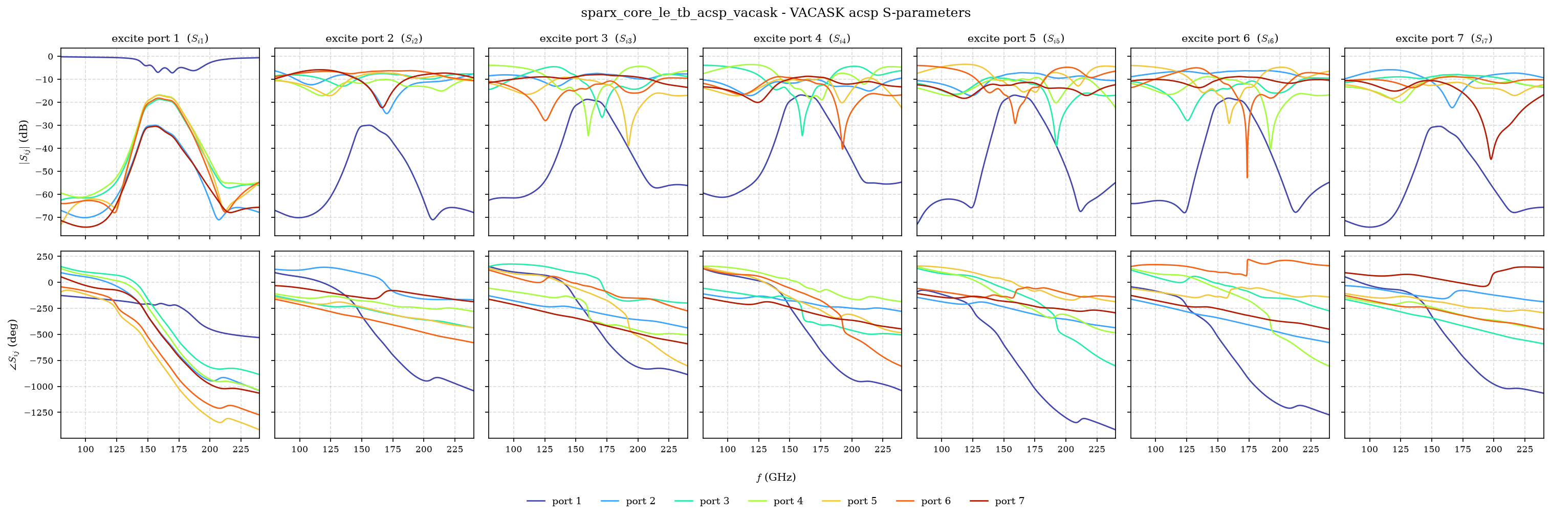
sparx_core_le_tb_acsp_vacask).
- The order-24 full-core fit reproduces the EM Touchstone at 160 GHz within 0.45 dB and 9.9° across all 49 S-parameters. Both extremes fall on one output-to-output coupling at -35 dB. Every other parameter is within 0.36 dB and 5°, and every one above -20 dB within 2.7°.
- The composed core reproduces the LO-path imbalances of the full-core solve within 0.4 dB and 5.5°, but overestimates the RF-path amplitude imbalance by up to 2.9 dB, because it contains neither the coupling between adjacent couplers nor the interconnects. It converges better and runs faster, which makes it the design-iteration model, while the full-core fit is the sign-off model.
- ngspice and VACASK agree within 0.001 dB on both models. That validates the two netlist dialects and nothing more, since both describe the same fit.
- The core’s thermal noise adds 0.0001 dB to the receiver noise figure, because 6 dB to 10 dB of passive loss sits in front of detectors with a 42 dB noise figure.
The passive benches sweep the band of testbenches/xschem/sim_range.inc and sim_range.spice, 80 GHz to 240 GHz, the band of the EM data. Outside it a vector fit extrapolates without data, so keep the benches inside the fitted band. In the deep BPF stopband, at -55 dB and below, a comparison in dB is meaningless. Compare in the passband or on a linear scale.
10 Circuit Simulation
10.1 Simulators and Analyses
Every passive model is simulated in both ngspice and VACASK, and the top-level transients run in both as independent integrators. The active characterization needs VACASK, since ngspice has no large-signal periodic analysis.
| Analysis | What it computes | Used for |
|---|---|---|
op, dc |
operating point, dc sweep | bias check in every bench |
acsp |
S-parameters from an AC analysis with ports | the ten passive-model benches |
noise |
small-signal noise at the dc operating point | detector NEP, reference noise figure without the LO |
tran |
transient, optionally with device noise | receiver waveforms, transient-noise ladders |
hb |
harmonic balance, single or multi-tone | detector transfer curve, receiver levels, the large-signal state under hbac and hbnoise |
pss |
periodic steady state by shooting | independent check of the HB transfer curve, the large-signal state under pac and pnoise |
hbac, pac |
small-signal transfer around the HB or PSS solution, sideband to sideband | conversion gain, video response, IF response |
hbnoise, pnoise |
small-signal noise around the HB or PSS solution, modulated and folded | detector and receiver noise figure with the LO on |
HB and shooting PSS compute the same periodic steady state with algorithms that share no code: HB solves for the Fourier coefficients, shooting for the initial condition that reproduces itself after one period. Agreement between the two, and between their small-signal and noise extensions, shows that a result is not an artifact of one algorithm. Transient noise shares no linearization with either.
10.2 Running Testbenches
make sim-xschem TB=sparx_bpf_le_tb_acsp_ngspice    # one bench
make sim-all                                       # every bench, in the right order
make sim-view-xschem SCRIPT=plot_n_port_tb_acsp_ngspice
sim-xschem saves the schematic, exports the netlist to testbenches/xschem/simulations/ and runs the simulator in batch mode. The name suffix selects the dialect and the simulator: _ngspice benches are netlisted as SPICE and run with ngspice -b, _vacask benches as Spectre and run with vacask -qp -sp, after which the Makefile runs the post-processing script of the bench. Results land in plot_simulations/data/ as CSV and JSON and in plot_simulations/figures/ as PNG. sim-view-xschem replots them on screen.
| Group | What is simulated | Benches |
|---|---|---|
| Passive models, S-parameters | BPF, WPD, BLC, full-core fit and composed core, each in ngspice and VACASK | 10 |
| Passive models, transient | stability and causality of the fits | 3 |
| SBD power detector | two-tone HB, transfer curve, noise figure, transient noise, ngspice cross-check | 6 |
| Receiver and top level | receiver characterization, receiver noise figure and transient noise, top-level transients | 5 |
The testbench README documents every bench: its analyses and settings, its findings and its limits. Some benches read the results of others, and sim-all runs them in the required order. The detector PSS bench runs before the detector NF bench, which reads the fitted responsivity. The receiver NF bench runs after the detector NF bench and the receiver bench. The transient-noise benches run after the NF benches whose results they check. The fits in netlist/ must exist before any bench that includes them.
10.3 Traps Worth Knowing
- Every 160 GHz transient needs a maximum time step. Without it, Gear integration in ngspice takes steps of about 0.3 ps on the carrier, damps it, and the IF comes out twelve times too small in a run that looks healthy. The ngspice benches use 20 fs, the VACASK receiver transient 50 fs.
- A symbol without
spectre_formatis dropped from a VACASK netlist without a warning, and the netlist still simulates. Every symbol in the repository carries it. - VACASK exits 0 when an analysis aborts or is unknown to the binary. Read the transcript for
aborted,failedornot found. - VACASK is case sensitive where ngspice is not, so
VSSandvssare two nodes. - An HB solution past 1 dB compression is not converged at nine harmonics. On the detector, nine harmonics overstated the conversion by 8.4 dB at +4 dBm of LO. The detector’s LO sweeps therefore run with 15 harmonics and are checked against
psswithpacandpnoise. - A shooting PSS on the full-core fit needs a first stabilization step of 20 fs or more. At the default of a thousandth of the period the stabilization transient aborts at once. The benches use
stabstep=50f.
11 Receiver Simulation
11.1 Receiver Characterization
The receiver bench sparx_top_le_tb_rx_vacask combines the order-24 full-core fit, the four detectors, and the off-chip 5 pF on every output. It drives the LO at 159 GHz on \(P_1\) and the RF at 161 GHz on \(P_2\), both through 50 \(\Omega\) at the pads, so the outputs beat at a 2 GHz IF. The post-layout version, VARIANT=m1_pex, uses the extracted detectors.
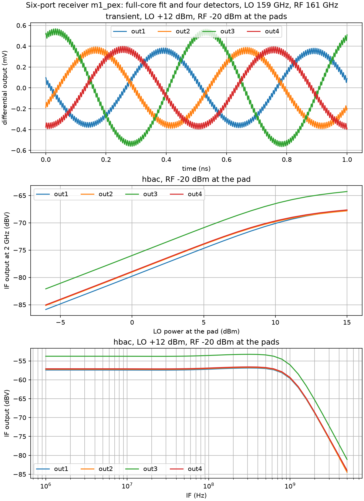
sparx_top_le_tb_rx_vacask, VARIANT=m1_pex).
- The LO path through BPF, WPD and BLC loses 17.3 dB to 18.6 dB into the detectors, so +12 dBm at the pad places the detectors at -6.6 dBm to -5.3 dBm, close to their noise-figure minimum of Section 6.4. The RF path through two BLCs loses 5.4 dB to 9.3 dB. These losses are into the post-layout detectors, whose input impedance differs from 50 \(\Omega\), so they differ from the 50 \(\Omega\) insertion loss of Section 8 by up to about 2 dB per output.
- The differences \(V_\mathrm{I}\) and \(V_\mathrm{Q}\) show an amplitude imbalance of 2.0 dB and a phase difference of 85.4° in the transient. The EM core terminated by the detector impedance gives 2.1 dB and 85.3°, so the circuit simulation of the receiver reproduces the EM within 0.1 dB and 0.1°. The same detector mismatch makes \(V_\mathrm{Q-}\) the largest of the four outputs.
- The IF amplitude rises by 1 dB per dB of LO up to about +9 dBm at the pad, where compression starts, and is 1 dB compressed at +10.7 dBm to +12 dBm.
- The transient reproduces the HBAC amplitudes within 0.2 dB, and a two-tone HB reproduces them within 0.5 dB.
11.2 Receiver Noise Figure
The noise-figure bench sparx_top_le_tb_nf_vacask evaluates the double-sideband noise figure of the four detector outputs and of the I and Q outputs, referred to the RF pad, through the full-core fit, which carries the core’s own thermal noise. It runs the small-signal noise at the dc operating point, HBNOISE and PNOISE, as fabricated and post-layout. The transient-noise ladder, the fourth estimate, runs in sparx_top_le_tb_tn_vacask on the fabricated detectors.
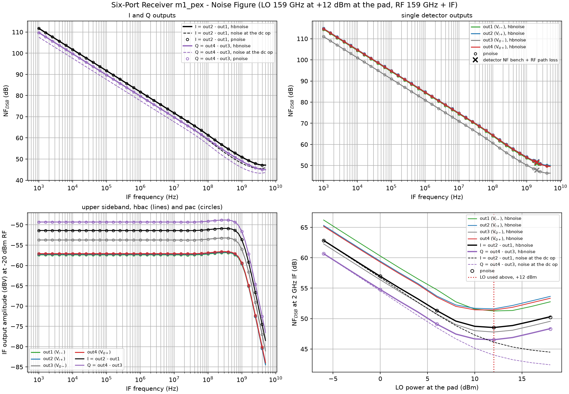
sparx_top_le_tb_nf_vacask, VARIANT=m1_pex).
| Output, 2 GHz IF, +12 dBm LO at the pad | HBNOISE, fabricated | HBNOISE, post-layout |
|---|---|---|
| \(V_\mathrm{I-}\), \(V_\mathrm{I+}\), \(V_\mathrm{Q-}\), \(V_\mathrm{Q+}\) | 48.3 dB to 52.6 dB | 47.8 dB to 51.6 dB |
| I | 48.5 dB | 48.5 dB |
| Q | 46.3 dB | 46.5 dB |
- I and Q are 1.3 dB to 2.7 dB better than their single detectors, since the signals of a pair add coherently in the difference while their noise adds in power.
- The LO source noise largely cancels in I and Q, because it reaches both detectors of a pair through the same LO path.
- Each detector output equals the noise figure of the detector bench at the LO drive that detector sees, plus its RF path loss, within 0.3 dB, once both refer to the power delivered into the detector.
- The minimum against LO drive lies at +10 dBm to +12 dBm at the pad. Below it the noise figure falls by 1 dB per dB of LO, the square-law regime: at +2 dBm and +4 dBm on the pad, the range of a probe-fed LO, the I output reads 55.1 dB and 53.2 dB post-layout.
- PNOISE reproduces HBNOISE within 0.1 dB, and the small-signal noise at the dc operating point is 2.1 dB to 3.3 dB optimistic, as on the single detector.
12 Regression and Continuous Integration
make regression is the smoke test of the tools and the flow in the IIC-OSIC-TOOLS environment, not a design sign-off. It needs nothing but a plain container and runs build-top with the add-on install, klayout-verify and magic-verify of the detector, the S-parameter copy and both snp2le conversions of the WPD, and one ngspice and one VACASK WPD bench. It reuses the committed WPD Palace result. make regression-full adds the WPD Palace solve.
| Workflow | Trigger | What it runs |
|---|---|---|
regression.yml |
push to main, and on manual dispatch |
make regression-full in hpretl/iic-osic-tools:latest |
license-check.yml |
push and pull request to main |
reuse lint |
quarto-publish.yml |
push to main, and on manual dispatch |
renders this documentation and publishes it to gh-pages |
The regression is also part of the release tests of the IIC-OSIC-TOOLS container, which validate every image against real designs.
13 Tapeout, Releases and Measurements
Bare dies of the March 2026 tapeout (RFFE6027) are back from fabrication. Figure 17 shows one, in the orientation of the pinout render in Figure 8.
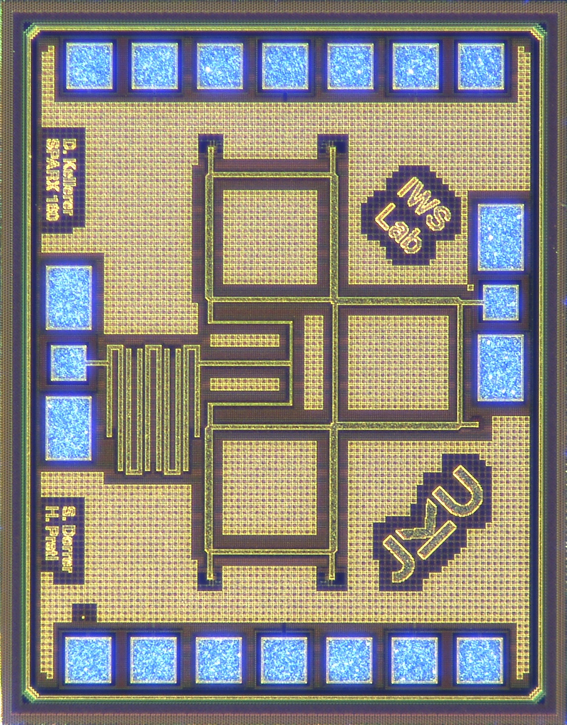
RFFE6027 (1 × 1.4 mm²).
| Release | Content |
|---|---|
release/v.1.0.0/ |
the March 2026 tapeout on the IHP open MPW run: RFFE6027.gds (1 × 1.4 mm²), its renders and the die photo. The submission repository is davkel99/IHP__RFFE6027 |
release/v.2.0.0/ |
a later export of the generator: sparx160_top.gds, netlists and renders |
make release VERSION=<version> copies the top-level GDS, the schematic and layout netlists and the renders into release/v.<version>/.
The measurement plan probes the LO and RF pads with a wafer prober and bonds the supply and detector pads to a PCB, read with an oscilloscope. A revised design is planned with 16-cell detectors, an optimized BPF, and active blocks such as an LNA, a VCO and an LO amplifier to compensate the LO-path loss.
14 Known Issues and Limitations
- Top-level LVS is open, blocked by IHP-Open-PDK issue 1041. Only the power detector has full LVS.
- Antenna rules.
klayout-drc-regularreports the 33 antenna violations IHP waived for the tapeout, see Table 15. - Author label. Every generated layout carries the label “SPARX 160”, whatever its frequency, because the label is a fixed image,
scripts/assets/D_Kellerer.png, placed as a committed GDS. - BPF. The closed-form models reach their limits on the meanders and coupled lines of the hairpin filter: the 160 GHz filter loses 10 dB and matches only to -6.2 dB, in the LO path. It is the block with the most to gain from optimization.
- No mesh-convergence study. The committed Palace runs use element order 2 on a single mesh without adaptive refinement. The metal-model check of Section 8.3 refined the TopMetal2 edges once, from 2 \(\mu\)m to 0.5 \(\mu\)m, which lowered the loss by 2 % to 6 %.
- Metal model. The EM runs use gds2palace’s surface metal model. Against volume physics the 50 \(\Omega\) lines read 6 % to 14 % too lossy and the BPF about 0.5 dB, while the WPD agrees within 1 %, see Section 8.3.
- Fit extrapolation. The fits see the EM band from 80 GHz to 240 GHz only, and they are passive inside it. Above it the WPD fit reaches a largest singular value of 1.618 at 679 GHz. The receiver benches also evaluate the core at the IF and at the LO harmonics, where the passive fit extrapolates. The detector noise figure plus the RF path loss, a composition in which the detector sees 50 \(\Omega\) at every frequency, agrees with the simulated receiver within 0.3 dB, which bounds the effect at the operating point.
- Detector noise model. 97 % of the detector noise comes from the flicker model of a parasitic PNP evaluated far below any characterized current, and its value depends on the BJT area scaling of the simulator build. Measurements will show how far it applies.
- Detector guard rings. The substrate guard rings of the two Schottky diodes are not tied to ground by metal. The
vssnetwork of the full-RC extraction therefore comes out differently in every run (extresistreports an orphaned node), and the VACASK benches idealize that net.
The repository keeps KNOWN_ISSUES.md and ToDo.md up to date.
15 Code-a-Chip Notebook
sscs-ose-code-a-chip/ holds a Jupyter notebook for the IEEE SSCS Open-Source Ecosystem Code-a-Chip Travel Grant Awards at ISSCC 2027, which runs in Google Colab. It installs the IHP Open-PDK and the GDSFactory add-on, generates the complete receiver from the design frequency, runs the KLayout DRC of the chip, converts the EM result of the core with snp2le, characterizes the detector and the post-layout receiver in VACASK, and simulates the receiver noise figure through the noisy core fit. It downloads VACASK fb8cc20 and OpenVAF-Reloaded as image layers of the IIC-OSIC-TOOLS 2026.10 image from Docker Hub, the first image with pac and pnoise, and applies the image’s fixes of the PDK model converter before it generates the model libraries. The five VACASK netlists it runs are plain exports of the repository’s testbenches, stored in testbenches/xschem/netlists/ for environments without Xschem. The notebook keeps its own copies of the GDS and assets and is not driven by the Makefile.
17 Cite This Work
Please cite the paper and the repository:
@inproceedings{Dorrer_2026,
  author    = {Dorrer, Simon and Kellerer-Pirklbauer, David and Zachl, Georg
               and Pretl, Harald},
  title     = {{SPARX: An Open-Source, Automated, Programmatically Generated,
               Frequency-Scalable Six-Port Receiver in 130-nm CMOS}},
  booktitle = {IEEE Nordic Circuits and Systems Conference (NorCAS)},
  year      = {2026},
  note      = {Accepted for publication}
}

@misc{2026_SPARX,
  author = {Dorrer, Simon and Kellerer-Pirklbauer, David and Pretl, Harald},
  month  = oct,
  year   = {2026},
  title  = {{GitHub Repository of SPARX: An Open-Source, Automated, Programmatically
            Generated, Frequency-Scalable Six-Port Receiver in 130-nm CMOS}},
  url    = {https://github.com/iic-jku/SG13CMOS_SPARX},
  doi    = {10.5281/zenodo.19654232}
}
18 Acknowledgements
This project is funded by the JKU/SAL IWS Lab, a collaboration of Johannes Kepler University and Silicon Austria Labs.

|

|
19 License
Licensed under the Solderpad Hardware License v2.1 (Apache-2.0 WITH SHL-2.1), see LICENSE.