Appendix: 5T-OTA Small-Signal Output Impedance

Analog (Integrated) Circuit Design

18 Appendix: 5T-OTA Small-Signal Output Impedance

Appendix: 5T-OTA Small-Signal Output Impedance

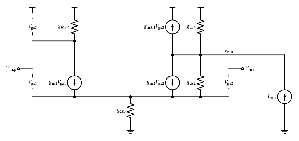
Figure 84: 5-transistor OTA small-signal model for output impedance calculations.

This section gives additional details to the analysis presented in Section 8.3. Here we provide the full calculation of the output impedance/conductance of the 5T-OTA for frequencies below the dominant pole, i.e., we neglect any capacitors.

18.1 Open-Loop Configuration

Open-Loop Configuration

For the open-loop case, the gates of \(M_1\) and \(M_2\) are tied to ground (and since \(M_1\) and \(M_2\) are matched \(g_\mathrm{m1} = g_\mathrm{m2} = g_\mathrm{m1,2}\)), which means that the gate-source voltages of \(M_1\) and \(M_2\) are identical: \[ V_\mathrm{in,p} = V_\mathrm{in,n} = 0 \to V_\mathrm{gs1} = V_\mathrm{gs2} = V_\mathrm{gs1,2} \tag{66}\]

\[ I_\mathrm{out} - g_\mathrm{ds4} V_\mathrm{out} - g_\mathrm{m3,4} V_\mathrm{gs3} - I_{g_\mathrm{ds2}} - g_\mathrm{m1,2} V_\mathrm{gs1,2} = 0 \tag{67}\]

KCL at the output node:

Open-Loop Configuration

KCL at the tail node: \[ 2 g_\mathrm{m1,2} V_\mathrm{gs1,2} + I_{g_\mathrm{ds2}} + g_\mathrm{ds5} V_\mathrm{gs1,2} = 0 \]

\[ I_{g_\mathrm{ds2}} = -\left( 2 g_\mathrm{m1,2} + g_\mathrm{ds5} \right) V_\mathrm{gs1,2} \tag{68}\]

We can solve for \(I_{g_\mathrm{ds2}}\).

Furthermore, we need an expression for \(V_\mathrm{gs3}\). Ohm’s law at the transconductance \(g_\mathrm{m34}\) will suffice.

Open-Loop Configuration

\[ V_\mathrm{gs3} = -\frac{g_\mathrm{m1,2}}{g_\mathrm{m3,4}} V_\mathrm{gs1,2} \tag{69}\]

\[ V_\mathrm{gs1,2} = -\frac{g_\mathrm{ds2}}{2 g_\mathrm{m1,2} + g_\mathrm{ds2} + g_\mathrm{ds5}} V_\mathrm{out} \tag{70}\]

KVL from the output node down to ground (traversing \(g_\mathrm{ds2}\) and \(g_\mathrm{ds5}\)) in combination with Equation 68 gives us an expression for \(V_\mathrm{gs1,2}\)

Now, we can plug in all quantities into Equation 67. First, Equation 68 is inserted, which provides an expression for the current through the output conductance \(g_\mathrm{ds2}\) of \(M_2\):

Open-Loop Configuration

\[ I_\mathrm{out} - g_\mathrm{ds4} V_\mathrm{out} - g_\mathrm{m3,4} V_\mathrm{gs3} + \left( g_\mathrm{m1,2} + g_\mathrm{ds5} \right) V_\mathrm{gs1,2} = 0 \]

\[ I_\mathrm{out} - g_\mathrm{ds4} V_\mathrm{out} + \left( 2 g_\mathrm{m1,2} + g_\mathrm{ds5} \right) V_\mathrm{gs1,2} = 0 \]

Second, \(V_\mathrm{gs3}\) is substituted by Equation 69. Since we have assumed a matched pair of transistors for the current mirror comprised of \(M_3\) and \(M_4\), \(g_\mathrm{m3,4}\) perfectly cancels out of the equation, and is effectively replaced by the transconductance \(g_\mathrm{m1,2}\) of the input transistor \(M_1\):

Third, Equation 70 gives us an expression for the last remaining unknown \(V_\mathrm{gs1,2}\). Thus, the factor in front of \(V_\mathrm{out}\) defines the conductance at the output node.

Open-Loop Configuration

\[ I_\mathrm{out} - \left[ g_\mathrm{ds4} + \left( 2 \cdot g_\mathrm{m1,2} + g_\mathrm{ds5} \right) \frac{g_\mathrm{ds2}}{2 g_\mathrm{m1,2} + g_\mathrm{ds2} + g_\mathrm{ds5}} \right] V_\mathrm{out} = 0 \tag{71}\]

\[ I_\mathrm{out} - \left[ g_\mathrm{ds4} + \frac{g_\mathrm{ds2} \cdot \left( 2\cdot g_\mathrm{m1,2} + g_\mathrm{ds5} \right)}{g_\mathrm{ds2} + \left( 2 \cdot g_\mathrm{m1,2} + g_\mathrm{ds5} \right)} \right] V_\mathrm{out} = 0 \tag{72}\]

Before we interpret this result, we slightly rearrange the equation to give us more insight:

Now, we can identify the common equation of the total resistance of two parallel resistors. However, we are dealing with conductances here, so the same equation describes the total conductance of two conductances in series, while parallel conductances are simply summed. In parallel to \(g_\mathrm{ds4}\), there is effectively the series connection of \(g_\mathrm{ds2}\) and \(2 \cdot g_\mathrm{m1,2} + g_\mathrm{ds5}\) at work.

If we apply the general assumption of \(g_\mathrm{m}\gg g_\mathrm{ds}\), only the parallel connection of \(g_\mathrm{ds4}\) and \(g_\mathrm{ds2}\) remains:

Open-Loop Configuration

\[ \frac{I_\mathrm{out}}{V_\mathrm{out}} \approx g_\mathrm{ds4} + g_\mathrm{ds2} \tag{73}\]

18.2 Closed-Loop Configuration

Closed-Loop Configuration

\[ V_\mathrm{in,n} = V_\mathrm{out} \quad \text{and} \quad V_\mathrm{in,p} = 0 \tag{74}\]

\[ I_\mathrm{out} - g_\mathrm{ds4} V_\mathrm{out} - g_\mathrm{m3,4} V_\mathrm{gs3} - g_\mathrm{ds2} V_\mathrm{gs2} - g_\mathrm{m1,2} V_\mathrm{gs2} = 0 \tag{75}\]

In contrast to the open-loop case, we keep the gate of \(M_1\) connected to ground and tie the input of \(M_2\) to the output node \(V_\mathrm{out}\):

KCL at the output node:

We use KVL from the output node down to ground to find an expression for \(V_\mathrm{gs2}\).

Closed-Loop Configuration

\[ V_\mathrm{gs2} = V_\mathrm{out} + V_\mathrm{gs1} \tag{76}\]

\[ g_\mathrm{m1,2} V_\mathrm{gs1} + g_\mathrm{m1,2} V_\mathrm{gs2} + g_\mathrm{ds2} V_\mathrm{gs2} + g_\mathrm{ds5} V_\mathrm{gs1} = 0 \tag{77}\]

KCL at the tail node:

Using Equation 76 to substitute \(V_\mathrm{gs2}\) in Equation 77 we find an equation for \(V_\mathrm{gs1}\):

Closed-Loop Configuration

\[ V_\mathrm{gs1} = -\frac{g_\mathrm{m1,2} + g_\mathrm{ds2}}{2 g_\mathrm{m1,2} + g_\mathrm{ds2} + g_\mathrm{ds5}} V_\mathrm{out} \tag{78}\]

\[ I_\mathrm{out} -\left( g_\mathrm{ds4} + g_\mathrm{ds2} + g_\mathrm{m1,2} \right) V_\mathrm{out} - g_\mathrm{m3,4} V_\mathrm{gs3} - \left( g_\mathrm{ds2} + g_\mathrm{m1,2} \right) V_\mathrm{gs1} = 0 \]

Again, we derive the output conductance by plugging Equation 76, Equation 69 and Equation 78 step by step into Equation 75. First, we use Equation 76 to eliminate \(V_\mathrm{gs2}\):

Second, Equation 69 also holds for the closed-loop case and lets us eliminate \(V_\mathrm{gs3}\):

Closed-Loop Configuration

\[ I_\mathrm{out} -\left( g_\mathrm{ds4} + g_\mathrm{ds2} + g_\mathrm{m1,2} \right) V_\mathrm{out} - g_\mathrm{ds2} V_\mathrm{gs1} = 0 \]

Third, we use Equation 78 to eliminate the remaining unknown \(V_\mathrm{gs1}\):

Closed-Loop Configuration

\[ \begin{split} & I_\mathrm{out} - \left( g_\mathrm{ds4} + g_\mathrm{ds2} + g_\mathrm{m1,2} \right) V_\mathrm{out} \\ &+ g_\mathrm{ds2} \frac{g_\mathrm{m1,2} + g_\mathrm{ds2}}{2 g_\mathrm{m1,2} + g_\mathrm{ds2} + g_\mathrm{ds5}} V_\mathrm{out} = 0 \end{split} \]

A simpler result can be obtained if we neglect \(g_\mathrm{ds2}\) and \(g_\mathrm{ds5}\) in Equation 78 (\(g_\mathrm{m}\gg g_\mathrm{ds}\)):

Closed-Loop Configuration

\[ I_\mathrm{out} -\left( g_\mathrm{ds4} + \frac{1}{2} g_\mathrm{ds2} + g_\mathrm{m1,2} \right) V_\mathrm{out} \approx 0 \]

\[ I_\mathrm{out} - g_\mathrm{m1,2} V_\mathrm{out} \approx 0 \to \frac{I_\mathrm{out}}{V_\mathrm{out}} \approx g_\mathrm{m1,2} \]

If we apply \(g_\mathrm{m}\gg g_\mathrm{ds}\) again we arrive at:

Closed-Loop Configuration