Economy of Integrated Circuits

Design of Complex Integrated Circuits

7 Economy of Integrated Circuits

7.1 Selling Price and Total Cost

The manufacturing of ICs is a large-scale business, requiring significant investment in research and development, and usually large volumes are built and sold. It is therefore rewarding to take a look at the economics of integrated circuits.

Selling Price and Total Cost

\[ S_\mathrm{tot} = \frac{C_\mathrm{tot}}{1 - m} \tag{57}\]

The selling price \(S_\mathrm{tot}\) of a good depends on the achievable profit margin \(m\) and the total cost of the product \(C_\mathrm{tot}\):

Selling Price and Total Cost

Table 11: Impact of the profit margin on the required selling price

Profit margin	Selling price
30 %	\(S_\mathrm{tot} \approx 1.4 \cdot C_\mathrm{tot}\)
50 %	\(S_\mathrm{tot} = 2 \cdot C_\mathrm{tot}\)
70 %	\(S_\mathrm{tot} \approx 3.3 \cdot C_\mathrm{tot}\)

The total cost \(C_\mathrm{tot}\) of a product consists of the non-recurring engineering cost (NRE) \(F'_\mathrm{tot}\) plus other fixed costs \(F''_\mathrm{tot}\) (together \(F_\mathrm{tot} = F'_\mathrm{tot} + F''_\mathrm{tot}\)), and the recurring cost \(R_\mathrm{tot}\). The recurring cost is incurred per IC, whereas NRE and fixed costs relate to the whole project; their impact on the cost per piece thus depends on the number of pieces sold, \(N_\mathrm{sold}\):

Selling Price and Total Cost

\[ C_\mathrm{tot} = R_\mathrm{tot} + \frac{F_\mathrm{tot}}{N_\mathrm{sold}} \tag{58}\]

7.2 Non-Recurring Engineering Cost

Non-Recurring Engineering Cost

\[ F'_\mathrm{tot} = E_\mathrm{tot} + P_\mathrm{tot} + I_\mathrm{tot} \tag{59}\]

The NRE consists of the engineering cost \(E_\mathrm{tot}\), the prototype cost \(P_\mathrm{tot}\), and the cost of licensed IP blocks \(I_\mathrm{tot}\):

Engineering cost: \(E_\mathrm{tot}\) depends on the size of the design team (architecture, design, simulation, layout, timing, DRC & tapeout, test). It includes salaries, benefits, training, computers, and CAD tool licenses. License costs can be substantial in IC design; approximate yearly costs per seat are $10k/yr for a digital front-end seat, $1M/yr for a digital back-end seat, and $100k/yr for an analog front-/back-end seat.

Prototype cost: The mask cost depends heavily on the process technology and the used technology options (e.g., additional \(V_\mathrm{th}\) flavors, analog options like precision resistors or MIM capacitors), which drive up the number of masking steps; see Table 12. A multi-project wafer (MPW), where multiple designs share a single reticle and thus the share also the mask cost, is a good alternative for prototypes. Also test fixtures (sockets, PCBs) and package tooling belong to \(P_\mathrm{tot}\).

Non-Recurring Engineering Cost

Table 12: Approximate mask-set costs for different technology nodes

Technology	Estimated mask-set cost
CMOS 180 nm	$80k
CMOS 28 nm	$1.5M
CMOS 5 nm	> $10M

IP cost: Large SoCs might require licensing of certain IP blocks (interfaces, processor cores, memory, etc.); patent licensing might be required as well. Types of licensed IP are:

Non-Recurring Engineering Cost

• Hard IP: circuit blocks defined at the mask (layout) and transistor (netlist) level.
• Firm IP: logic-level/register netlist.
• Soft IP: described at the register-transfer level (RTL) in an HDL.

Licensed cores must come with documentation, BIST, a test-pattern delivery method, or external test patterns.

Other fixed costs \(F''_\mathrm{tot}\) include datasheets and application notes, marketing and advertising, and yield analysis and production support.

7.3 Recurring Cost

Recurring Cost

\[ R_\mathrm{tot} = R_\mathrm{die} + R_\mathrm{pack} + R_\mathrm{test} \tag{60}\]

The recurring cost consists of the fabrication cost per IC, considering the wafer manufacturing, packaging, and test:

The packaging cost \(R_\mathrm{pack}\) depends mainly on the type of package and the packaging yield. The test cost \(R_\mathrm{test}\) depends strongly on the type of tester (digital, mixed-signal, RF) and the test time (the duration of the test program including robotic handling); an effective way to reduce test cost is to test several devices in parallel.

7.3.1 Dice per Wafer

\[ R_\mathrm{die} = \frac{W}{N \cdot Y} \tag{61}\]

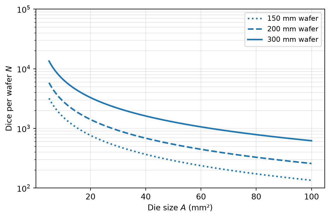
\[ N \approx d \pi \left( \frac{d}{4 A} - \frac{1}{\sqrt{2 A}} \right) \tag{62}\]

The cost per die depends strongly on the cost per wafer \(W\) (on the order of $500 to $30,000), the die area \(A\), the usable wafer diameter \(d\) (nominal wafer diameter minus twice the edge exclusion), and the yield \(Y\):

The edge exclusion (EE) is the ring around the circumference where no functional IC can be placed, typically 2 to 3 mm (we use 2 mm here). The number of dice per wafer can be approximated by (\(A\) in mm², \(d\) in mm) (Vries 2005)

which is plotted in Figure 69 for the standard wafer sizes.

Dice per Wafer

Figure 69: Number of dice per wafer as a function of the die size, for the standard wafer diameters (2 mm edge exclusion assumed).

7.3.2 Yield

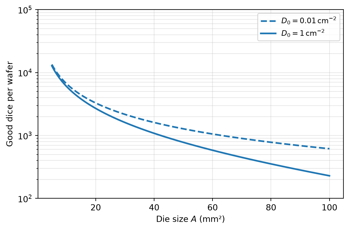
\[ Y = \left( \frac{1 - e^{- A D_0}}{A D_0} \right)^2 \approx e^{-A D_0} \tag{63}\]

The yield \(Y\) is the number of functional dice divided by the total number of dice per wafer (\(Y = 50\,\%\) means that half of the produced ICs are defective). Wafer processing incurs a defect density per unit area (\(D_0 \approx 0.01\) to \(1\,\text{cm}^{-2}\)) in the silicon structures—this is why clean rooms and careful processing are essential. The defect density and the die area are related to the yield by Murphy’s model (Murphy 1964):

Equation 63 shows that the die size is also a critical factor for yield! Combining Equation 62 and Equation 63 yields the number of good dice per wafer, depicted in Figure 70.

Yield

Figure 70: Good dice per wafer versus die size for a 300 mm wafer (2 mm edge exclusion) and two defect densities, using the simplified Murphy yield model of Equation 63.

7.4 An Exemplary Calculation

An Exemplary Calculation

Note 5: IC Cost and Selling Price

Let us calculate the required selling price for an IC using the following assumptions:

Parameter	Value
Wafer cost \(W\) for a \(d = 200\,\text{mm}\) wafer	$1500
Die size \(A\)	15 mm²
Yield \(Y\)	95 %
Targeted gross margin \(m\)	50 %
NRE plus fixed cost \(F_\mathrm{tot}\)	$5M
Package and test cost	$0.75

Using Equation 62 with \(d = 196\,\text{mm}\) (2 mm edge exclusion), we get \(N \approx 1900\) dice per wafer, and with Equation 61, the cost per die is

\[ R_\mathrm{die} = \frac{\$1500}{1900 \cdot 0.95} = \$0.83 \]

The total recurring cost per die is (using Equation 60)

\[ R_\mathrm{tot} = \$0.83 + \$0.75 = \$1.58 \]

The required selling price is strongly dependent on the number of ICs sold (using Equation 57 and Equation 58):

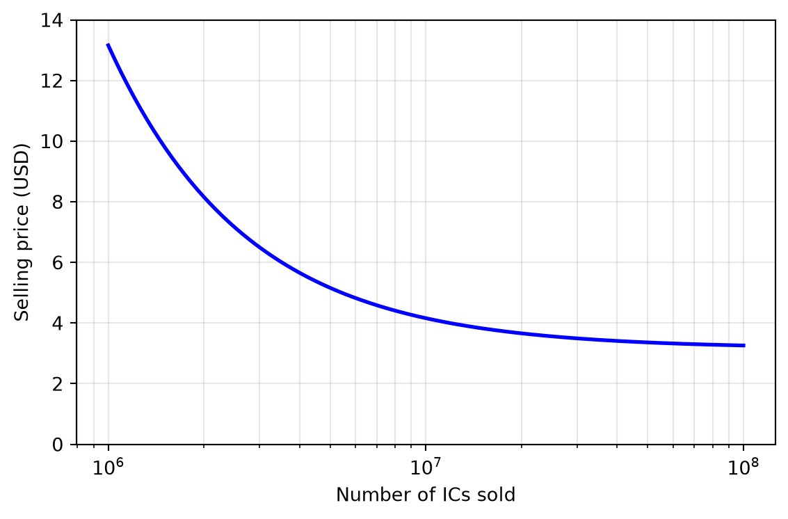
\[ S_\mathrm{tot} = \frac{1}{1 - m} \left( R_\mathrm{tot} + \frac{F_\mathrm{tot}}{N_\mathrm{sold}} \right) = 2 \left( \$1.58 + \frac{\$5\,\text{M}}{N_\mathrm{sold}} \right) \]

An Exemplary Calculation

IC Cost and Selling Price

The resulting selling price versus sales volume is plotted in Figure 71: in the left region (low volume), the fixed cost \(F_\mathrm{tot}\) dominates the selling price, whereas for larger volumes the recurring cost \(R_\mathrm{tot}\) becomes crucial.

An Exemplary Calculation

IC Cost and Selling Price

Figure 71: Required selling price versus sales volume for this exemplary IC: at low volumes, the fixed costs dominate; at high volumes, the price approaches twice the recurring cost.

References

Murphy, Bernard T. 1964. “Cost-Size Optima of Monolithic Integrated Circuits.” Proceedings of the IEEE 52 (12): 1537–45. https://doi.org/10.1109/PROC.1964.3442.

Vries, Dirk K. de. 2005. “Investigation of Gross Die Per Wafer Formulas.” IEEE Transactions on Semiconductor Manufacturing 18 (1): 136–39. https://doi.org/10.1109/TSM.2004.836656.

In the example of Note 5, we can clearly see that at low sales volumes, the fixed costs dominate the selling price, whereas at high sales volumes, the selling price approaches twice the recurring cost. Since a fixed-cost dominated IC product is often simply too expensive, it is crucial to achieve sufficient sales volume to make the product economically viable.

References