Mixers

Radio-Frequency Integrated Circuits

5 Mixers

Mixers

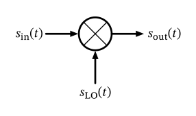
Figure 41: Mixer block diagram.

As we have seen in Section 3.2, we are using mixers to “upconvert” and “downconvert” signals, i.e., we shift the frequency of a signal to a higher or lower frequency with the help of an auxiliary signal, called the “local oscillator” (LO) signal. The block diagram of a mixer is shown in Figure 41.

Mixers

\[ \omega_\mathrm{out} = \omega_\mathrm{in} \pm \omega_\mathrm{LO}. \]

What we usually want in a mixer is that the input signal at \(\omega_\mathrm{in}\) is shifted by \(\omega_\mathrm{LO}\), so that the output signal is located at

It should be noted that the output signal usually contains additional frequency components, which are not desired. These so-called “spurious” components are usually filtered out in a subsequent filtering stage.

Recalling the properties of linear time-invariant (LTI) systems, we know that in an LTI system no new frequency components (which are not already present in the input signal) are generated. In conclusion, in order to generate new frequency components, a mixer has to be either

Mixers

• a non-linear system, or
• a time-variant system.

Next we will look at two options on how to implement a mixer.

5.1 Non-Linear Mixer

Non-Linear Mixer

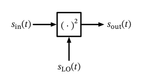
Figure 42: A squarer as a nonlinear mixer.

Generally speaking, we can use any nonlinear device to implement a mixer (often, this generation of new frequency components in a nonlinear system is highly undesired; in a mixer, we want this effect). As a simple example we look at the case of a square function, shown in Figure 42.

Non-Linear Mixer

\[ \begin{split} s_\mathrm{out}(t) = [ s_\mathrm{in}(t) + s_\mathrm{LO}(t) ]^2 &= \cos(\omega_\mathrm{in} t + \omega_\mathrm{LO} t) + \cos(\omega_\mathrm{in} t - \omega_\mathrm{LO} t) \\ &+ 1 + \frac{1}{2} \cos(2 \omega_\mathrm{in} t) + \frac{1}{2} \cos(2 \omega_\mathrm{LO} t). \end{split} \tag{50}\]

When we apply the sum of the signals \(s_\mathrm{in}(t) = \cos( \omega_\mathrm{in} t)\) and \(s_\mathrm{LO}(t) = \cos(\omega_\mathrm{LO} t)\) to the input of a squarer, we get the output signal

We see that the output signal contains the desired frequency components at \(\omega_\mathrm{in} \pm \omega_\mathrm{LO}\), but also additional components at dc (0 Hz), \(2 \omega_\mathrm{in}\), and \(2 \omega_\mathrm{LO}\). These additional components are usually unwanted and have to be filtered out in a subsequent filtering stage. As a side-note, in some circuits a frequency doubler is desired, which can be implemented by simply filtering out the other frequency components. In a doubler no LO signal is required, as the input signal is simply squared.

A simple example circuit is a diode, which has a non-linear current-voltage characteristic. The block diagram of a simple diode mixer is shown in Figure 43.

Non-Linear Mixer

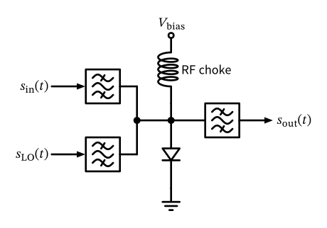
Figure 43: A diode mixer.

5.2 Time-Variant Mixer

This structure is conceptually simple; it just requires a (fast) diode, filters to couple the desired frequency components in and out, and an RF choke to provide a dc bias voltage for the diode. However, the performance of such a simple mixer is usually not very good, as the diode is a highly non-linear device, which generates many spurious frequency components. More advanced mixer circuits use more complex non-linear devices (for example, a ring of diodes) to improve the performance. The advantage of these mixers is that they can operate up to very high frequencies (in the mm-wave range and beyond). If you can make a nonlinear device, you can make a mixer (think also of nonlinear optics, for example).

Time-Variant Mixer

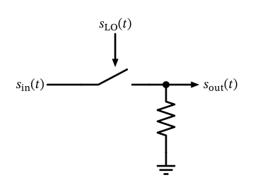
Figure 44: A switch as a time-variant mixer.

In contrast to the non-linear mixer, a time-variant mixer uses an ideally linear device, but changes its properties over time. A simple example is a switch, which is opened and closed at the LO frequency. The block diagram of such a mixer is shown in Figure 44. This system is ideally linear from input to output, but very nonlinear when considering the LO input.

Time-Variant Mixer

\[ \begin{split} s_\mathrm{out}(t) &= s_\mathrm{in}(t) \cdot \underbrace{\frac{1}{2} \left\{ 1 + \mathrm{sgn}[ s_\mathrm{LO}(t) ] \right\}}_\text{Fourier series} \\ &= s_\mathrm{in}(t) \cdot \left[ \frac{1}{2} + \frac{2}{\pi} \sin(\omega_\mathrm{LO} t) + \frac{2}{3 \pi} \sin(3 \omega_\mathrm{LO} t) + \frac{2}{5 \pi} \sin(5 \omega_\mathrm{LO} t) + \ldots\right] \end{split} \]

When the switch is closed (\(s_\mathrm{LO} \ge 0\)), the input signal is passed to the output, i.e., \(s_\mathrm{out}(t) = s_\mathrm{in}(t)\); when the switch is open (\(s_\mathrm{LO} < 0\)), no signal is passed, i.e., \(s_\mathrm{out}(t) = 0\). The output signal can be expressed as

where \(\mathrm{sgn}(\cdot)\) is the signum function. The term in curly brackets is a square wave that switches between 0 and 1 at the LO frequency. This square wave can be expressed as a Fourier series, which contains the fundamental frequency at \(\omega_\mathrm{LO}\) and all odd harmonics \(3 \omega_\mathrm{LO}\), \(5 \omega_\mathrm{LO}\), and so on. In conclusion, if the input signal is expressed as \(\cos(\omega_\mathrm{in} t)\), we get the output signal

Time-Variant Mixer

\[ s_\mathrm{out}(t) = \frac{1}{\pi} \cos(\omega_\mathrm{in} t \pm \omega_\mathrm{LO} t) + \ldots \tag{51}\]

Again, we see that the output signal contains the desired frequency components at \(\omega_\mathrm{in} \pm \omega_\mathrm{LO}\), but also additional components at \(3 \omega_\mathrm{LO}\), \(5 \omega_\mathrm{LO}\), and so on. These additional components are usually unwanted and have to be filtered out in a subsequent filtering stage. The advantage of a time-variant mixer is that it can be implemented readily in CMOS, as shown in Figure 45.

Time-Variant Mixer

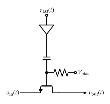
Figure 45: A MOSFET switch used as a mixer with an ac-coupled LO signal.

Time-Variant Mixer

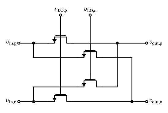
Figure 46: A fully-differential double-balanced MOSFET mixer.

The implementation in Figure 45 uses a single NMOS transistor as a switch. The LO signal is ac-coupled to the gate of the transistor, so that the dc operating point is set by the bias voltage \(V_\mathrm{bias}\). When the LO signal is high enough, the transistor is switched on and the input signal \(v_\mathrm{in}(t)\) is passed to the output; when the LO signal is low, the transistor is switched off and no signal is passed. Note that with the MOSFET we can switch voltages as well as currents, so the mixer can work in both modes, voltage mode or current mode.

A big disadvantage of this simple, unbalanced implementation is that the input signal is “lost” for half of the cycle when the MOSFET switch is open. A fully differential implementation (having differential ports at input, output and LO input) can alleviate this problem, as the input signal is always connected to one of the two output ports. This configuration is called a “double-balanced mixer” and is widely used in practice. It is shown in Figure 46.

Time-Variant Mixer

\[ s_\mathrm{out}(t) = \frac{2}{\pi} \cos(\omega_\mathrm{in} t \pm \omega_\mathrm{LO} t) + \ldots \tag{52}\]

The balanced structure changes the switching function from one toggling between 0 and 1 into one toggling between \(-1\) and \(+1\). The Fourier series of the latter has twice the fundamental amplitude, so the conversion gain doubles from \(1/\pi\) to \(2/\pi\), i.e., we gain 6 dB compared to the unbalanced mixer of Equation 51:

The factor \(2/\pi\) corresponds to a conversion loss of 3.9 dB, which is the best an ideal balanced passive mixer can do.

Time-Variant Mixer

Single-Balanced vs. Double-Balanced

The 6 dB are not due to double balancing: a single-balanced mixer already realizes the \(\pm 1\) switching function and the \(2/\pi\) conversion gain. Double balancing adds port-to-port isolation: LO and RF feedthrough in Figure 46 are common-mode at the output and thus suppressed.

Take care not to attribute these 6 dB to the double-balancing itself. A single-balanced mixer (a single-ended input driving a differential pair of switches with a differential output) already realizes the \(\pm 1\) switching function, and therefore already achieves the \(2/\pi\) conversion gain. What the second level of balancing buys is port-to-port isolation: in the double-balanced mixer of Figure 46 both the LO feedthrough and the RF feedthrough appear as common-mode signals at the differential output and are thus suppressed. This is why the double-balanced structure is the workhorse in practice, not because of any additional conversion gain.

Time-Variant Mixer

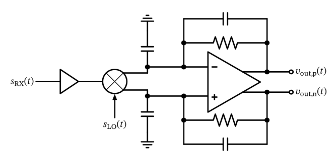
Figure 47: An RX front-end using a current-mode (passive) mixer.

Note that no dc current needs to flow through the mixer structures shown in Figure 45 and Figure 46, which is a huge advantage when thinking of flicker noise. Careful, though: this is not because the flicker noise of a MOSFET disappears without dc current. The gate-referred flicker noise \(K_f / (C'_\mathrm{ox}W L f)\) of Section 2.3.1 is independent of the bias current. What matters is that this gate-referred voltage noise is converted into a drain current noise, \(\overline{I_\mathrm{n,1/f}^2} = g_\mathrm{m}^2 K_f / (C'_\mathrm{ox}W L f)\), and it is this current that is translated to the mixer output. In a passive mixer the switches are driven hard on and off, and with (ideally) zero dc current through them there is no bias current for the flicker noise to modulate, so the contribution at the output is drastically reduced (Redman-White and Leenaerts 2001). This is in stark contrast to an active (Gilbert-type) mixer, where the switching pair carries the transconductor’s bias current at all times.

Passive mixers are therefore the architecture of choice for zero-IF receivers, where the downconverted signal sits right at dc and is thus maximally exposed to 1/f noise.

In order to look at the full picture, we embed the mixer of Figure 46 in a complete RX front-end, as shown in Figure 47. An LNA (essentially a \(g_\mathrm{m}\) cell) creates a current signal from the received voltage signal at the antenna. This current signal is then fed to the mixer in the current domain, and further sunk into a transimpedance amplifier (TIA), which also implements a lowpass pole. The simplified circuit is shown in Figure 47.

5.3 Gilbert Cell Mixer

The capacitors connected directly to ground at the mixer outputs are good practice, as they shunt high-frequency switching noise to ground, and in this way help the performance of the TIA, which otherwise would have to sink these currents. Note that all blocker currents originating at the LNA output and passing through the mixer are shunted by the feedback capacitors to the output of the TIA, and need to be actively driven by the TIA’s output stage!

Gilbert Cell Mixer

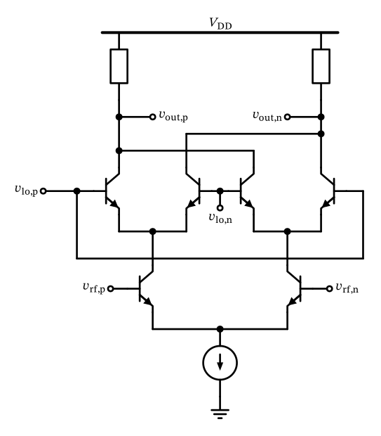
Figure 48: A Gilbert mixer based on bipolar differential pairs.

As we have seen in Section 5.2, in CMOS we have quite a few options to implement a mixer as the MOSFET is a good current and voltage switch. This is in stark contrast to the BJT, as the bipolar transistor can only be used as an (excellent) current switch in the differential pair configuration. Hence, we need to implement a current-mode mixer in bipolar technology. The most widely used structure is the so-called “Gilbert cell”, shown in Figure 48.

5.4 N-Path Filter

The idea is that an input transconductor creates currents, which are switched in the double differential pair and converted back to voltage in the load impedances. There are many known variations of this circuit, like skipping the current source at the bottom to increase linearity and headroom, or swapping the input transconductor for another structure. It might also be useful to “bleed” some bias current from the LO switching stage to improve the noise performance.

N-Path Filter

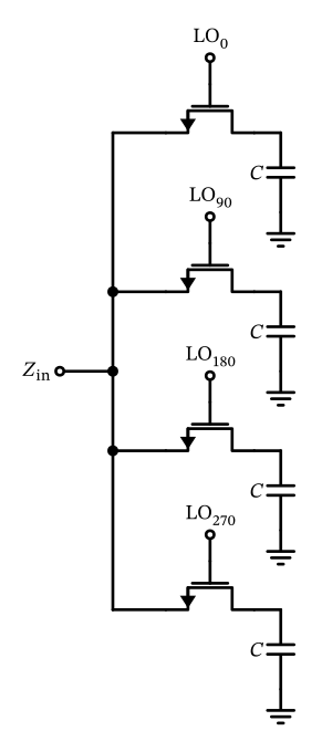
Figure 49: A 4-phase N-path filter.

Without much deliberation or diving into the background, it has to be stated that passive mixers (based on MOSFET switches) have a few very interesting properties. One of them is that they can be used to implement very high-quality bandpass filters, called “N-path filters” (Lepage et al. 1953). The basic idea is shown in Figure 49. We use four phases of an LO signal to switch the four capacitors to ground in a round-robin fashion. The duty cycle of each LO phase is 25% to have a non-overlapping clock.

N-Path Filter

\[ Z_\mathrm{in}(\omega_\mathrm{LO} + \Delta \omega) \approx R_\mathrm{sw} + Z_\mathrm{BB}(\Delta \omega), \tag{53}\]

The key observation to make is that a switch that is opened and closed at a certain frequency (the LO frequency) can be seen as a time-variant resistor. This time-variant resistor converts impedance seen at one end to the other end, and also changes the frequency of this apparent impedance. In other words, if we connect grounded capacitors at one end of the mixer switches and look into the other end, we see a bandpass filter centered at the LO frequency! In this way we can build bandpass filters (and also bandstop filters (Vazny et al. 2010)) at very high frequencies which are precisely centered (without component variations) around \(\omega_\mathrm{LO}\).

The reason this works is the transparency of the passive mixer: the impedance connected to the baseband side of the switches appears at the RF port, frequency-shifted to \(\pm \omega_\mathrm{LO}\). If the baseband load is a first-order \(RC\) section with impedance \(Z_\mathrm{BB}(\Delta \omega)\), then the RF-port impedance around the LO is simply

i.e., a first-order bandpass centered exactly at \(\omega_\mathrm{LO}\), sitting on top of the series switch resistance \(R_\mathrm{sw}\). This is shown in Figure 50. Two properties follow directly from Equation 53 and make the N-path filter so attractive:

N-Path Filter

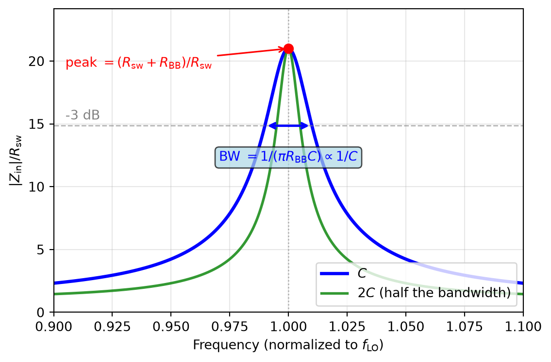
• The peak impedance is \(R_\mathrm{sw} + R_\mathrm{BB}\), where \(R_\mathrm{BB}\) is the effective shunt resistance at baseband. The switch resistance therefore sets the floor of what is achievable — low-\(R_\mathrm{sw}\) switches are essential.
• The bandwidth is inversely proportional to the capacitance, \(\mathrm{BW} \propto 1/C\), while the center frequency is set solely by \(\omega_\mathrm{LO}\). This gives us a filter whose center frequency and bandwidth are independently and precisely programmable — something no passive \(LC\) filter can offer. The resulting effective \(Q = \omega_\mathrm{LO}/\mathrm{BW}\) can easily reach several hundreds.

A detailed treatment, including the dependence on \(N\) and the duty cycle as well as the folding of the higher harmonics, can be found in (Ghaffari et al. 2011).

N-Path Filter

Figure 50: Input impedance of an N-path filter, obtained by frequency-translating the first-order baseband \(RC\) impedance to \(\pm f_\mathrm{LO}\) and adding the series switch resistance.

Input impedance of an N-path filter, obtained by frequency-translating the first-order baseband \(RC\) impedance to \(\pm f_\mathrm{LO}\) and adding the series switch resistance. Doubling the path capacitance halves the bandwidth, while the peak impedance stays at \(R_\mathrm{sw} + R_\mathrm{BB}\).

5.5 LO Generation

5.5.1 RC/CR Phase Shift Network

As you have seen in Section 3.2, for complex-valued modulation schemes (like QPSK, QAM, OFDM, and so on) we need to generate quadrature LO signals (i.e., two LO signals with a 90° phase shift). There are many ways to generate such signals, and we will now study a few of them.

Probably the simplest way to generate quadrature LO signals is to use a simple RC/CR phase shift network, as shown in Figure 51. The RC network (a first-order lowpass) generates a phase shift between 0° and -90°, while the CR network (a first-order highpass) generates a phase shift between 0° and +90°. By operating the network at \(\omega_0 = 1/RC\), we can achieve a 90° phase shift between the two outputs.

RC/CR Phase Shift Network

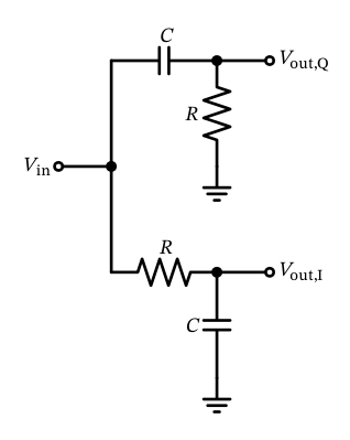
Figure 51: An RC/CR IQ generation network.

5.5.2 Polyphase Filter

The advantage of this network is its simplicity, as it only requires a few passive components, and it can generate I and Q phases from an incoming signal at the target frequency. The disadvantage is that both the phase shift and the amplitude are frequency-dependent: exactly at \(\omega_0 = 1/RC\) the two outputs are perfectly in quadrature and have equal magnitude (\(1/\sqrt{2}\) each), but as soon as we move away from \(\omega_0\) the lowpass output rolls off while the highpass output rises, so we accumulate both a phase error and an amplitude imbalance. Since the resulting I/Q mismatch directly limits the image rejection (see Equation 29), this network is only usable over a narrow frequency range, and typically requires additional amplitude-limiting or gain stages. Additionally, this passive network has a 3 dB loss at \(\omega_0\), which also has to be made up by subsequent gain stages.

We can create a more advanced phase shift network (following the idea of Section 5.5.1) by using a so-called “polyphase filter” (Kaukovuori et al. 2008). The idea is to use multiple RC sections to create a more ideal phase shift network. An example is shown in Figure 52.

Polyphase Filter

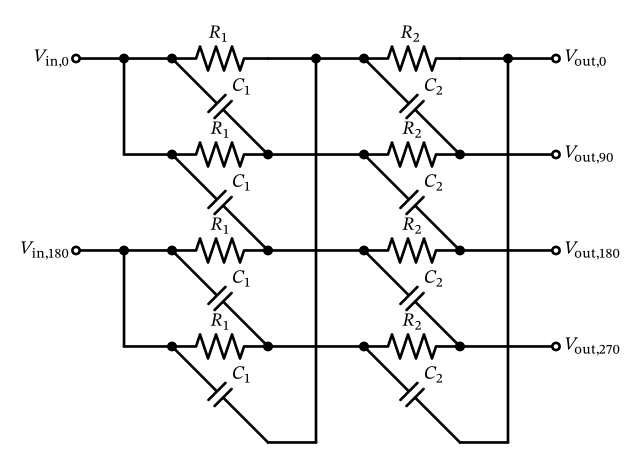
Figure 52: A two-stage polyphase network.

5.5.3 Flip-Flop Based Phase Generation

As shown in the figure above, we can use multiple stages (with \(R_1 C_1 \ne R_2 C_2\)) in cascade to broaden the frequency range over which we have a good 90° phase shift between the four outputs. The more stages we use, the better the performance, but also the more components are required. Note that this network is still passive, so it has an inherent loss, which also increases with the number of stages. The idea behind this network is that the network is transparent for positive frequencies, and blocks negative frequencies (or vice versa). We enter the network with real signals (having positive and negative frequency components), and at the output we get complex signals (having only positive or negative frequency components). In this sense this network is a complex filter.

Note that polyphase filters are popular when we have to create complex signals from real signals. We can use the polyphase filter in the LO path, or also in the signal path (e.g., in a receiver). The benefit is that we can work with a signal where the input frequency is equal to the output frequency. This is in strong contrast to the approach we will discuss next.

The most widely used approach to generate quadrature LO signals is to use digital circuits, as shown in Figure 53. The idea is to use a flip-flop (or a latch) to divide the frequency of an incoming clock signal by two. If we drive the two flip-flops (which are connected as toggle flip-flops) by inverted clocks, then the resulting output signals are 90° phase-shifted, as shown in Figure 54.

Flip-Flop Based Phase Generation

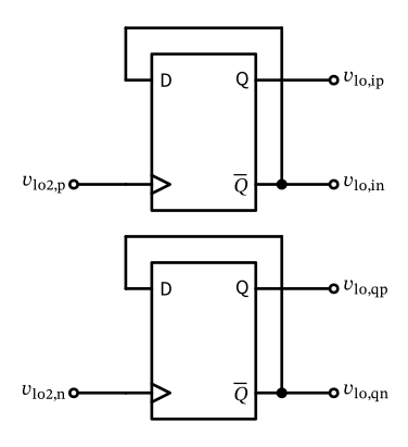
Figure 53: I/Q generation with a divide-by-2.

Flip-Flop Based Phase Generation

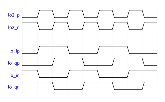
Figure 54: Input and output waveforms of I/Q generation with a divide-by-2.

Flip-Flop Based Phase Generation

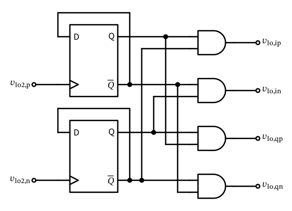
Figure 55: I/Q generation with a divide-by-2 and 25% duty cycle generation.

It is important to note that the circuit shown in Figure 53 has to be implemented in a way so that there is no phase ambiguity, i.e., the Q-phase is lagging the I-phase by exactly 90° (as drawn in Figure 54). This can be achieved by using a reset signal to set the flip-flops to a known state at startup, or by implementing flip-flops using a differential clock input.

If the input clock is not 2x the target frequency but higher (e.g., 4x), then we can use a frequency divider approach to generate more than four phases. This could be useful in an N-path filter, where we could need more than four phases (see Section 5.4).

Often, we need four-phase LO signals with 25% duty cycle (instead of the 50% duty cycle shown in Figure 54). This can be achieved by using additional logic gates to combine the outputs of the flip-flops, as shown in Figure 55. The resulting LO waveforms are shown in Figure 56.

Flip-Flop Based Phase Generation

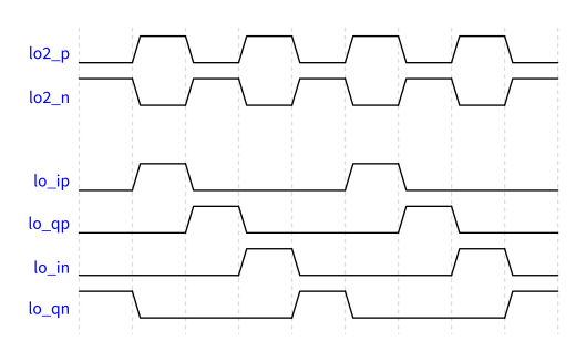
Figure 56: Input and output waveforms of I/Q generation with a divide-by-2 and 25% duty cycle generation.

5.5.4 Delay-Based Phase Generation

The advantage of using flip-flops to generate multi-phase LO signals is that very precise phase shifts can be achieved, which can be produced over a very wide frequency range. They can be implemented in different logic styles, like CMOS, ECL, CML, and so on. The disadvantage is that we need a high-frequency clock signal above the target frequency, which might be difficult to generate. Still, I/Q generation with flip-flops is the de-facto standard approach in modern RFICs.

The final approach we want to mention is to use a delay line (or multiple ones) to generate phase shifts. Using transmission lines, this approach is widely used at very high frequencies, where other approaches (like the ones shown in Section 5.5.2 or Section 5.5.3) are difficult to implement. One well-known approach is the 90° hybrid coupler, realized with \(\lambda/4\) transmission lines (Pozar 2011). When the frequencies are high enough (and the resulting wavelengths short enough), this approach can even be implemented on-chip. The disadvantage is that the phase shift is frequency-dependent, so the quadrature signals are only perfectly in quadrature at one frequency. Furthermore, this passive network has a 3 dB loss, so we need additional gain stages to compensate for this loss. A branch-line hybrid coupler is shown in Figure 57.

Delay-Based Phase Generation

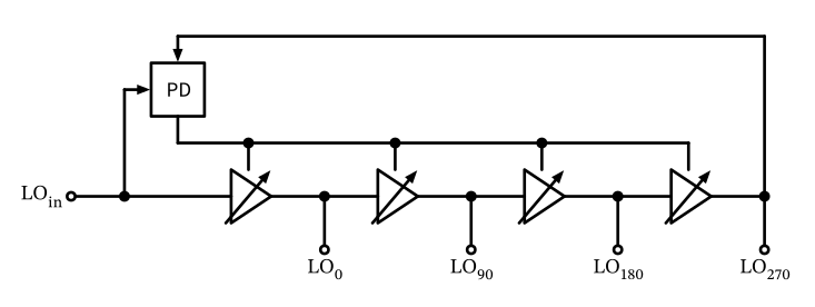
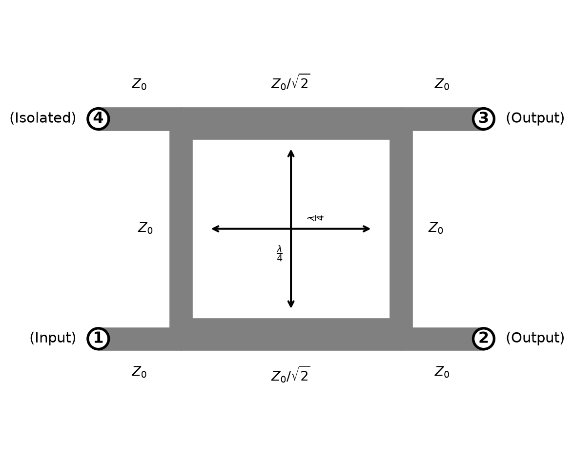
Figure 57: Branch-line hybrid coupler schematic showing the transmission line structure with characteristic impedances and λ/4 length sections.

Delay-Based Phase Generation

\[ S = \frac{1}{\sqrt{2}} \begin{bmatrix} 0 & -j & -1 \\ -j & 0 & 0 \\ -1 & 0 & 0 \end{bmatrix}. \tag{54}\]

The 3-port S-parameter matrix of an ideal branch-line coupler (assuming port 4 is properly terminated with \(Z_0\)) is given by

A feature of the coupler in Figure 57 is that it is single-ended; a differential implementation needs either two couplers or a coupler with subsequent baluns. An alternative implementation of a 90° hybrid coupler is the Lange coupler, which uses interdigitated fingers to achieve the required coupling. The Lange coupler can be implemented in a single-ended or differential way, and it can achieve very good performance over a wide frequency range. The disadvantage is that it requires a large number of fingers, which can take up a lot of area on-chip (Lange 1969).

Another approach, which is similar to the flip-flop based approach, is to use a delay line to generate the required phase shifts. This can be done with a single delay line and multiple taps, or with multiple delay lines. The idea is that we delay the input clock signal by a certain amount of time, which corresponds to a 90° phase shift at the target frequency. This approach is shown in Figure 58. Since the delay of a delay line is frequency dependent, and the delay will change with process, voltage, and temperature (PVT) variations, we have to implement a tuning mechanism to adjust the delay. This implementation is called a delay-locked loop (DLL), which is similar to a phase-locked loop (PLL, see Section 7).

Delay-Based Phase Generation

Figure 58: LO multiphase generation by delay-locked loop (DLL).

LO multiphase generation by delay-locked loop (DLL). An extension to more than four phases is straightforward.

References

Ghaffari, Amir, Eric A. M. Klumperink, Michiel C. M. Soer, and Bram Nauta. 2011. “Tunable High-Q N-Path Band-Pass Filters: Modeling and Verification.” IEEE Journal of Solid-State Circuits 46 (5): 998–1010. https://doi.org/10.1109/jssc.2011.2117010.

Kaukovuori, Jouni, Kari Stadius, Jussi Ryynänen, and Kari A. I. Halonen. 2008. “Analysis and Design of Passive Polyphase Filters.” IEEE Transactions on Circuits and Systems–I: Regular Papers 55 (10): 3023–37. https://doi.org/10.1109/tcsi.2008.917990.

Lange, J. 1969. “Interdigitated Strip-Line Quadrature Hybrid.” 1969 g-MTT International Microwave Symposium, 10–13. https://doi.org/10.1109/GMTT.1969.1122649.

Lepage, W. R., C. R. Cahn, and J. S. Brown. 1953. “Analysis of a comb filter using synchronously commutated capacitors.” Transactions of the American Institute of Electrical Engineers, Part I: Communication and Electronics 72 (1): 63–68. https://doi.org/10.1109/tce.1953.6371974.

Pozar, David M. 2011. Microwave Engineering. 4th edition. Wiley.

Redman-White, William, and Dominicus Martinus Wilhelmus Leenaerts. 2001. “1/f Noise in Passive CMOS Mixers for Low and Zero IF Integrated Receivers.” Proceedings of the 27th European Solid-State Circuits Conference, 41–44. https://api.semanticscholar.org/CorpusID:32079786.

Vazny, Rastislav, Werner Schelmbauer, Harald Pretl, Stefan Herzinger, and Robert Weigel. 2010. “An Interstage Filter-Free Mobile Radio Receiver with Integrated TX Leakage Filtering.” 2010 IEEE Radio Frequency Integrated Circuits Symposium, January, 21–24. https://doi.org/10.1109/rfic.2010.5477294.

With a phase detector (PD) we can compare the phase of the output signal with the input signal, and regulate the delay per stage so that after four delays the edges line up. Then we can tap the equally-spaced phases and use them as LO signals. The advantage of this approach is that we can flexibly create a required number of phases from an input clock. This feature is also used in wireline communication systems to generate multiple phases for the data sampling.

References