Appendix: RF Circuit Simulation

Radio-Frequency Integrated Circuits

10 Appendix: RF Circuit Simulation

Appendix: RF Circuit Simulation

• Widely separated time scales: GHz LO, kHz to MHz signal, Hz flicker noise
• Large periodic signals (LO, clock, carrier): the circuit is time-variant for the small signal (Section 5.2)
• Frequency translation of noise: modulated and folded noise
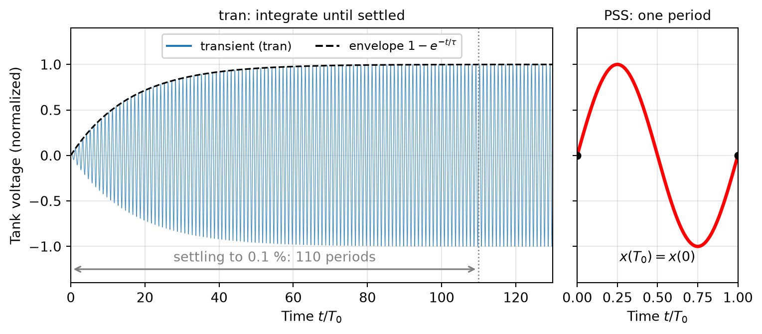
• High-Q resonators and oscillators: long settling, no stable dc operating point

There is no breadboard for an integrated circuit: every design decision in an RFIC is checked by circuit simulation before tapeout. A SPICE-type simulator (Nagel 1975) offers a small set of fundamental analyses (dc operating point, small-signal ac and noise, and transient), which are perfectly adequate for amplifiers, filters, and bias circuits. RF circuits, however, push these analyses to their limits, for several reasons:

• Widely separated time scales. An LO at several GHz carries information at kHz to MHz offsets, and flicker noise matters down to a few Hz. A time-domain simulation must resolve the fastest signal for as long as the slowest one needs.
• Large periodic signals. The LO of a mixer, the clock of a switched-capacitor filter, or the carrier of a PA moves the operating point periodically. With respect to the small signal, such a circuit is time-variant (see Section 5.2), so an analysis linearized around a constant operating point cannot capture its behavior.
• Frequency translation of noise. In such time-variant circuits, noise is modulated by the large signal and folded from many frequencies onto the wanted output frequency.
• High-Q resonators and oscillators. High-Q circuits take many periods to settle, and an oscillator has no stable dc operating point at all. Its frequency and phase noise are results of the large-signal operation.

Appendix: RF Circuit Simulation

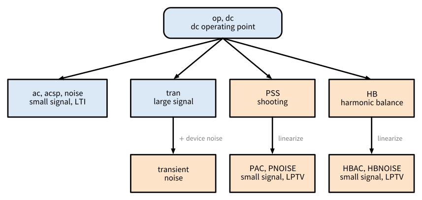
Figure 106: Family tree of circuit simulation analyses.

These challenges led to a set of advanced RF analyses: transient noise, periodic steady-state analysis by shooting (PSS) and by harmonic balance (HB), and the small-signal (PAC, HBAC) and noise (PNOISE, HBNOISE) analyses built on top of a periodic steady state (Kundert 1999). For a long time, the complete set was only available in commercial simulators, while open-source simulators offered parts of it (e.g., harmonic balance in Xyce, and transient-noise sources and an experimental oscillator PSS in ngspice). Since September 2026, the development version of the open-source simulator VACASK (Bűrmen 2025) supports all of them. The IIC-OSIC-TOOLS container ships them from its release 2026.10 on, so that the complete RF verification flow of this appendix can be run with open-source tools. The analysis names used in this appendix follow VACASK, which largely uses the names of Cadence Spectre (Spectre calls the operating point dc, the small-signal analysis ac and the S-parameter analysis sp, where VACASK uses op, ac and acsp). Section 10.4 lists the corresponding ngspice commands.

Figure 106 shows how the analyses build on each other. All of them start from the dc operating point. The small-signal analyses linearize the circuit either around this constant operating point, which gives a linear time-invariant (LTI) system, or around a periodic steady state, which gives a linear periodically time-varying (LPTV) system.

Family tree of circuit simulation analyses. Every analysis starts from the dc operating point. The small-signal analyses linearize around a constant operating point (LTI) or around a periodic steady state (LPTV). The periodic steady state is found either in the time domain (shooting PSS) or in the frequency domain (harmonic balance, HB). The fundamental analyses are shown in blue, the advanced RF analyses in orange.

Appendix: RF Circuit Simulation

\[ \mathbf{f}(\mathbf{x}(t)) + \frac{\mathrm{d}}{\mathrm{d}t} \mathbf{q}(\mathbf{x}(t)) = \mathbf{u}(t), \tag{70}\]

All analyses solve the same circuit equations. With modified nodal analysis (MNA), a circuit is described by

where the vector \(\mathbf{x}\) contains the unknown node voltages and selected branch currents (of inductors and voltage sources), \(\mathbf{f}\) the currents of the resistive elements (summed per node according to Kirchhoff’s current law) together with the branch equations of voltage sources and inductors, \(\mathbf{q}\) the charges of capacitors and fluxes of inductors, and \(\mathbf{u}\) the independent sources. The analyses differ only in the assumption they make about \(\mathbf{x}(t)\):

• dc operating point: all time derivatives vanish, \(\mathbf{f}(\mathbf{x}_0) = \mathbf{u}_\mathrm{DC}\).
• ac and noise: a small deviation from \(\mathbf{x}_0\), so that Equation 70 can be linearized around \(\mathbf{x}_0\) (LTI).
• transient: no assumption at all. The time derivative is discretized, and Equation 70 is integrated step by step.
• PSS and HB: the solution is periodic, \(\mathbf{x}(t + T) = \mathbf{x}(t)\) (or quasi-periodic for several incommensurate tones in HB).
• PAC, PNOISE, HBAC, HBNOISE: a small deviation from a periodic steady state \(\mathbf{x}_\mathrm{s}(t)\), so that Equation 70 can be linearized around \(\mathbf{x}_\mathrm{s}(t)\) (LPTV).

Appendix: RF Circuit Simulation

• op: \(\mathrm{d}/\mathrm{d}t = 0\), \(\mathbf{f}(\mathbf{x}_0) = \mathbf{u}_\mathrm{DC}\)
• ac, noise: linearized around \(\mathbf{x}_0\) (LTI)
• tran: no assumption, integrate in time
• PSS, HB: \(\mathbf{x}(t + T) = \mathbf{x}(t)\)
• PAC, PNOISE, HBAC, HBNOISE: linearized around \(\mathbf{x}_\mathrm{s}(t)\) (LPTV)

10.1 Fundamental Analyses

10.1.1 DC Operating Point and DC Sweep

\[ \mathbf{G}(\mathbf{x}^{(i)}) \, \Delta \mathbf{x}^{(i)} = \mathbf{u}_\mathrm{DC} - \mathbf{f}(\mathbf{x}^{(i)}), \qquad \mathbf{x}^{(i+1)} = \mathbf{x}^{(i)} + \Delta \mathbf{x}^{(i)}, \tag{71}\]

The operating point analysis (op) sets all time derivatives in Equation 70 to zero (capacitors become open circuits, inductors short circuits) and solves the remaining nonlinear algebraic equations \(\mathbf{f}(\mathbf{x}_0) = \mathbf{u}_\mathrm{DC}\) with the Newton-Raphson method. Starting from an initial guess \(\mathbf{x}^{(0)}\), it iterates

where \(\mathbf{G} = \partial \mathbf{f} / \partial \mathbf{x}\) is the Jacobian (the conductance matrix of the linearized circuit). Each iteration requires the solution of a sparse linear system. Newton-Raphson converges very fast close to the solution but can fail from a poor starting point. Simulators therefore fall back to continuation methods such as gmin stepping (temporarily adding conductances to ground) or source stepping (ramping up the supplies). The same Newton iteration is the inner engine of every other analysis in this appendix.

A dc sweep (.dc in ngspice, a sweep around op in VACASK) repeats the operating point analysis while stepping a source or a parameter, using each solution as the starting point of the next one. It yields static transfer characteristics, e.g., the dc output of a power detector versus a bias voltage, or the multiplier characteristic of a Gilbert cell (Section 5.3).

DC Operating Point and DC Sweep

Always Check the Operating Point First

Every small-signal analysis (ac, acsp, noise) linearizes around the operating point and inherits all its errors. Check bias currents, \(g_\mathrm{m}/I_\mathrm{D}\) values, and saturation margins before looking at any other result. Note also that circuits with positive feedback (latches, oscillators) have an operating point that is an unstable equilibrium: it is a valid solution of the equations, but the real circuit never stays there.

DC Operating Point and DC Sweep

Always Check the Operating Point First

For bistable circuits, the operating point may not converge at all, and a defined state (a reset or a nodeset) helps.

10.1.2 Small-Signal AC Analysis

\[ \left( \mathbf{G} + j \omega \mathbf{C} \right) \mathbf{X}(j\omega) = \mathbf{U}(j\omega), \qquad \mathbf{G} = \frac{\partial \mathbf{f}}{\partial \mathbf{x}}, \quad \mathbf{C} = \frac{\partial \mathbf{q}}{\partial \mathbf{x}}, \tag{72}\]

The ac analysis (ac) assumes a small sinusoidal excitation, \(\mathbf{x}(t) = \mathbf{x}_0 + \mathrm{Re}\{\mathbf{X} e^{j \omega t}\}\), and linearizes Equation 70 around the operating point. In the frequency domain, this gives one complex linear system per frequency:

with both Jacobians evaluated at \(\mathbf{x}_0\). As the system is linear, the amplitude of the source is arbitrary (usually 1 V), and the results are transfer functions: gain, phase, bandwidth, input and output impedances, and the loop gain of feedback circuits (for stability). An ac sweep is very fast, as it requires only one sparse linear solve per frequency point.

By construction, the ac analysis cannot show any distortion, compression, or frequency conversion: the response appears only at the excitation frequency.

10.1.3 S-Parameter Analysis

\[ a_i = \frac{V_i + Z_0 I_i}{2 \sqrt{Z_0}}, \quad b_i = \frac{V_i - Z_0 I_i}{2 \sqrt{Z_0}}, \quad S_{ij} = \frac{b_i}{a_j} \quad (a_k = 0 \text{ for } k \neq j). \tag{73}\]

The S-parameter analysis (acsp in VACASK, .sp in ngspice) is an ac analysis with ports. Each port is an excitation source with a reference impedance \(Z_0\) (usually 50 Ω). With the voltage \(V_i\) and the current \(I_i\) flowing into port \(i\), the incident and reflected power waves and the scattering parameters are (Pozar 2011)

For an amplifier, \(S_{11}\) describes the input match (return loss, see Equation 32), \(S_{21}\) the gain, \(S_{12}\) the reverse isolation, and \(S_{22}\) the output match. From the same data, the stability factors \(K\) and \(\mu\) follow directly (Equation 34 and Equation 36). S-parameters are also the natural description of passive structures like inductors, transformers, couplers, and filters, which are usually characterized by electromagnetic (EM) field simulation and enter the circuit simulation as Touchstone data or as fitted lumped-element models.

10.1.4 Small-Signal Noise Analysis

\[ S_\mathrm{out}(f) = \sum_i \left| H_i(f) \right|^2 S_i(f), \tag{74}\]

The noise analysis (noise) models every noise source of the circuit (thermal noise of resistors and channels, shot noise of junctions, flicker noise, see Section 2.3.1) as a stationary random source, whose power spectral density (PSD) \(S_i(f)\) is evaluated at the dc operating point. For uncorrelated sources, the contributions add in power at the output

where \(H_i(f)\) is the small-signal transfer function from source \(i\) to the output. Correlated sources, such as the induced gate noise and the channel noise of a MOSFET (see Section 2.3.1), add cross terms, which the simulator takes into account. Simulators either solve the linearized circuit once per noise source, or obtain all \(H_i(f)\) at once from a single adjoint (transposed) solve per frequency. The results are the output noise PSD, the input-referred noise (dividing by the gain), and, most valuable for design, a ranking of the contributions of every device and every noise mechanism. The noise factor (Equation 21) follows as the ratio of the total output noise to the part contributed by the source resistance alone. A load resistor that only models the next stage must be excluded from the output noise, as its noise is not part of the circuit under test.

The noise analysis is the standard tool for LNAs, baseband amplifiers, TIAs, and bias and reference circuits. Its key assumption, however, is a constant operating point. In a circuit driven by a large periodic signal, the noise sources are modulated by the signal, and noise from many frequencies is translated to the output frequency. A plain noise analysis of a mixer, a sampling circuit, or an oscillator is therefore wrong, as we will see in Section 10.2.5.

10.1.5 Transient Analysis

\[ \mathbf{f}(\mathbf{x}_{n+1}) + \frac{\mathbf{q}(\mathbf{x}_{n+1}) - \mathbf{q}(\mathbf{x}_n)}{h_n} = \mathbf{u}(t_{n+1}), \tag{75}\]

The transient analysis (tran) makes no assumption about the waveforms. It discretizes time, \(t_{n+1} = t_n + h_n\), and replaces the time derivative in Equation 70 with a numerical integration formula. With the simplest one, the backward Euler method, the equations at the new time point become

which is solved for \(\mathbf{x}_{n+1}\) with the Newton iteration of Equation 71. Practical simulators use the trapezoidal rule or the Gear (backward differentiation) formulas of second order, and adapt the time step \(h_n\) by estimating the local truncation error.

The transient analysis is the most general one: it handles any nonlinearity, any waveform, start-up, settling, and digital control. It is therefore the reference that all other analyses can be checked against. Its drawbacks in RF circuits are:

• Cost. The number of time points is the simulated time divided by the step size. The step size is set by the fastest signal (the LO or RF carrier and its edges), the simulated time by the slowest effect (settling of high-Q networks and bias circuits, the IF signal, and the frequency resolution \(1/T_\mathrm{sim}\) of a subsequent FFT).
• Numerical artifacts. The trapezoidal rule can show spurious ringing, while the Gear formulas add numerical damping, which can make an oscillator die out or attenuate a high-frequency carrier. A maximum time step that resolves the carrier is therefore mandatory. In a 160 GHz receiver testbench, for example, omitting it let the Gear integrator damp the carrier, and the IF output came out twelve times too small in a run that finished quickly and looked healthy (Dorrer et al. 2026).
• Spectral analysis. Distortion and spurs require an FFT of a waveform in steady state, with coherent sampling or windowing, resampled to a uniform time grid, and with simulator tolerances tight enough that the numerical noise floor lies well below the products of interest.

Transient Analysis

• Cost: step size set by the fastest signal, simulated time by the slowest effect
• Numerical artifacts: trapezoidal ringing, Gear damping, so always set a maximum time step that resolves the carrier
• Spectral analysis: needs steady state, coherent sampling or windowing, and tight tolerances

Transient Analysis

Note 9: Transient Simulation Effort of a Mixer

We want to simulate the conversion gain of a downconversion mixer with \(f_\mathrm{LO} = 2.4\,\text{GHz}\) and an IF around 1 MHz, with a frequency resolution of 10 kHz. The simulated time must be at least

\[ T_\mathrm{sim} \geq \frac{1}{10\,\text{kHz}} = 100\,\mu\text{s}. \]

With 50 time points per LO period, the step size is \(h = 1 / (50 \cdot 2.4\,\text{GHz}) \approx 8.3\,\text{ps}\), and we need

\[ N = \frac{T_\mathrm{sim}}{h} = 100\,\mu\text{s} \cdot 50 \cdot 2.4\,\text{GHz} = 1.2 \cdot 10^{7} \]

Transient Analysis

Transient Simulation Effort of a Mixer

time points, each requiring a Newton solve of the full circuit, and this excludes the settling time. A PSS analysis of the same mixer integrates only a few tens of LO periods (\(10^3\) to \(10^4\) time points, depending on the time resolution per period), and the conversion gain then follows from a PAC analysis with one linear solve per IF frequency (Section 10.2.4).

10.1.6 Comparison of the Fundamental Analyses

Table 8: Comparison of the fundamental analyses.

Analysis	Solves	Assumption	Typical RF use
op, dc sweep	\(\mathbf{f}(\mathbf{x}_0) = \mathbf{u}_\mathrm{DC}\)	static	bias point, dc transfer curves
ac	Equation 72	small signal, LTI	gain, bandwidth, impedances, loop gain
acsp	Equation 72 with ports	small signal, LTI	matching, gain, isolation, stability, passives
noise	Equation 74	small signal, stationary noise	NF of LNAs and baseband, noise contributions
tran	Equation 75	none	start-up, settling, switching, large-signal reference

10.2 Advanced RF Analyses

Advanced RF Analyses

1. Large-signal step. The periodic steady state is computed directly, either in the time domain (shooting PSS, Section 10.2.2) or in the frequency domain (HB, Section 10.2.3), without simulating the settling transient.
2. Small-signal step. The circuit is linearized around this periodic steady state. The resulting LPTV system is analyzed for frequency-translating transfer functions (PAC, HBAC, Section 10.2.4) and for cyclostationary noise (PNOISE, HBNOISE, Section 10.2.5).

The fundamental analyses either linearize around a constant operating point (ac, noise) or integrate the full nonlinear equations in time (tran). Many RF circuits sit in between: a large periodic signal, such as the LO of a mixer, the clock of a switched-capacitor (SC) filter or sampler, the carrier of a PA, or the oscillation itself in an oscillator, sets a periodically time-varying operating point, while the information-bearing signal and the noise are small. The advanced analyses exploit this structure in two steps:

Transient noise (Section 10.2.1) is the exception: it is a straightforward extension of the transient analysis, without any linearization.

10.2.1 Transient Noise

• Statistics: one realization per run, so long records, many seeds, resolution \(1/T_\mathrm{sim}\)
• Run time: step size limited by \(f_\mathrm{max}\)
• Band limits: flicker needs \(T_\mathrm{sim} \gg 1/f_\mathrm{min}\), resample finely before a PSD
• Numerical artifacts: run at reduced noise amplitudes, keep the part that scales with the amplitude squared
• Clocked circuits: complete all needed decisions, validate independently

In a transient noise simulation, every noise source of the circuit is replaced by a random time-domain waveform with the correct PSD within a band from \(f_\mathrm{min}\) to \(f_\mathrm{max}\), and injected into an ordinary transient analysis. White noise is generated from independent random samples, and flicker noise is approximated by a sum of filtered (Lorentzian) processes whose corner frequencies cover the band from \(f_\mathrm{min}\) to \(f_\mathrm{max}\). The samples are either held constant on a fixed time grid (zero-order hold) or integrated as stochastic differential equations along the actual time steps. To resolve the noise up to \(f_\mathrm{max}\), the time step is limited to a fraction of \(1/(2 f_\mathrm{max})\).

Because the circuit equations are integrated without linearization, transient noise includes in principle everything: switching, strong nonlinearity, sampling and noise folding, the conversion of noise into jitter, and even noise-induced decisions such as metastability and bit errors in comparators. In practice, it is also the numerically most fragile of all analyses, and the price is high:

• Statistics. Each run produces one random realization. A PSD, a jitter value, or an error probability requires long records, averaging, or many runs with different random seeds, and the frequency resolution is \(1/T_\mathrm{sim}\). A fixed seed reproduces a run only for an unchanged netlist, so after a circuit change, a difference within the scatter of the seeds is not a result.
• Run time. The step size is limited by \(f_\mathrm{max}\), even in parts of the waveform where the signal itself would allow large steps.
• Band limits. Flicker noise down to \(f_\mathrm{min}\) requires \(T_\mathrm{sim} \gg 1/f_\mathrm{min}\), and a default lower band edge derived from \(f_\mathrm{max}\) (in VACASK, \(f_\mathrm{max}/1000\)) can silently remove all flicker noise at the offsets of interest. When the noise is integrated along the actual time steps, white noise extends up to the Nyquist frequency of these steps. The waveform must then be resampled at least as finely as the simulator’s own steps before a PSD is computed, or out-of-band noise aliases into the band.
• Numerical artifacts. Device noise is tiny compared to the signals, and on stiff, strongly nonlinear circuits the random excitation itself can cause numerical errors that a noiseless run does not show. Run the analysis at two or more reduced noise amplitudes (a scaling factor such as noisescale in VACASK makes this easy), and use the part of the output noise power that scales with the square of the amplitude. Accept a higher-order part only if its size and order match a physical mechanism. A run at zero noise amplitude with otherwise identical settings, which uses the same time grid, shows the numerical floor.
• Clocked circuits. For comparators and sampled-data circuits, make sure that the run completes for the full number of decisions or cycles the statistics need, and validate the result against an independent estimate, such as an analytic \(kT/C\) budget or a periodic noise analysis.

10.2.2 Periodic Steady State by Shooting (PSS)

\[ \boldsymbol{\phi}_T(\mathbf{x}_0) - \mathbf{x}_0 = \mathbf{0}. \tag{76}\]

\[ \left( \mathbf{\Phi}_T - \mathbf{I} \right) \Delta \mathbf{x}_0 = \mathbf{x}_0 - \boldsymbol{\phi}_T(\mathbf{x}_0), \qquad \mathbf{\Phi}_T = \frac{\partial \boldsymbol{\phi}_T}{\partial \mathbf{x}_0}, \tag{77}\]

Typical applications are comparators (input-referred noise from the decision statistics: the dc input at which the output is zero in about 16 % of the decisions equals the rms input noise (Razavi 2020)), sampled-data circuits and ADCs (\(kT/C\) noise and the SNR including all effects), the jitter of oscillators, clock buffers, and dividers, and, increasingly important, an independent cross-check of PNOISE and HBNOISE results. Transient noise shares no solver code with the periodic analyses, but it uses the same device noise models. Their agreement therefore validates the implementation of the analyses rather than the noise models, and its statistics limit it to about a decibel.

Consider a circuit driven by large-signal sources with period \(T = 1/f_0\). After the start-up transient has died out, the circuit is in its periodic steady state \(\mathbf{x}_\mathrm{s}(t + T) = \mathbf{x}_\mathrm{s}(t)\). Let \(\boldsymbol{\phi}_T(\mathbf{x}_0)\) denote the state reached after integrating the circuit equations over one period, starting from the state \(\mathbf{x}_0\). The shooting method searches for the initial state that reproduces itself after one period (Aprille and Trick 1972):

This is again solved with Newton’s method,

where the sensitivity matrix \(\mathbf{\Phi}_T\) (the monodromy matrix) is computed alongside the transient integration over one period. Every Newton iteration therefore costs one period of transient simulation. For a linear circuit, the method converges in a single iteration, and a mildly nonlinear circuit needs a few. Usually, a short stabilization transient precedes the Newton loop to provide a good initial guess. In large circuits, the dense matrix \(\mathbf{\Phi}_T\) would be prohibitive, and matrix-free iterative (Krylov subspace) solvers made shooting practical for circuits with thousands of nodes (Telichevesky et al. 1995). VACASK currently integrates the full matrix \(\mathbf{\Phi}_T\), which is fine for circuit blocks but becomes expensive for large (e.g., post-layout) netlists.

The main advantage is illustrated in Figure 107: a high-Q circuit that needs many periods to settle in a transient analysis (about 110 for \(Q = 50\)) is solved with one or a few shooting iterations of one period each, because Newton’s method jumps directly to the steady state.

Periodic Steady State by Shooting (PSS)

Figure 107: Transient response of a resonator with \(Q = 50\) that is driven at its resonance frequency from \(t = 0\).

Transient response of a resonator with \(Q = 50\) that is driven at its resonance frequency from \(t = 0\). A transient analysis has to integrate about 110 periods until the amplitude is within 0.1 % of its final value. A PSS analysis solves for the single steady-state period (red) directly, and for this linear tank a single shooting iteration over one period suffices.

Periodic Steady State by Shooting (PSS)

PSS Does Not Prove Start-Up

PSS finds a periodic solution, but it does not tell whether the circuit actually reaches it after power-up. Whether an oscillator starts reliably over all corners (or whether a divider locks into the intended mode) must still be checked with a transient analysis.

Since the integration happens in the time domain with adaptive steps, PSS handles sharp edges and strongly nonlinear behavior just as well as a transient analysis: switching mixers, SC circuits, frequency dividers, rectifiers, and switching PAs (class D, E, F). Its main limitation is that it needs a single period: all large-signal sources must be periodic with a common period \(T\). A two-tone test with tones at 2.400 GHz and 2.401 GHz, for example, has a common period of 1 µs, i.e., 2400 carrier periods, which makes shooting inefficient. Note that only the large signals count: a small RF signal handled by PAC (Section 10.2.4) does not enter the period.

For oscillators (autonomous circuits), the period is unknown and becomes an additional unknown of the Newton iteration. As any time-shifted copy of a periodic solution is also a solution, a phase condition is added to make the problem well-defined. An autonomous PSS directly delivers the oscillation frequency and the steady-state waveform, without simulating the start-up. The circuit has to be kicked away from its (unstable) dc operating point by an initial condition, otherwise the analysis converges to the trivial dc solution.

10.2.3 Harmonic Balance (HB)

\[ \mathbf{x}(t) = \sum_{k=-K}^{K} \mathbf{X}_k \, e^{j k \omega_0 t}, \qquad \mathbf{X}_{-k} = \mathbf{X}_k^{*}, \tag{78}\]

\[ \mathbf{F}_k(\mathbf{X}) + j k \omega_0 \, \mathbf{Q}_k(\mathbf{X}) = \mathbf{U}_k, \qquad k = -K, \ldots, K. \tag{79}\]

From the periodic waveforms, the Fourier coefficients follow directly: harmonic distortion, the dc shift of a rectifier or power detector, the duty cycle of an LO signal, the efficiency of a PA (from the output power at the fundamental and the averaged supply power), and, for oscillators, frequency and amplitude versus a tuning voltage (i.e., the tuning curve and \(K_\mathrm{VCO}\), see Section 6.6).

Harmonic balance describes every unknown by a truncated Fourier series with \(K\) harmonics (not to be confused with the stability factor \(K\) of Section 4.2),

and solves for the Fourier coefficients \(\mathbf{X}_k\) directly (Nakhla and Vlach 1976). Inserted into Equation 70, the time derivative becomes an exact multiplication by \(j k \omega_0\), and the circuit equations must hold (“balance”) at every harmonic:

Here, \(\mathbf{F}_k\) and \(\mathbf{Q}_k\) are the Fourier coefficients of \(\mathbf{f}(\mathbf{x}(t))\) and \(\mathbf{q}(\mathbf{x}(t))\). Nonlinear device equations cannot be evaluated in the frequency domain, so HB transforms the present estimate of the spectrum into the time domain (inverse FFT), evaluates the devices at the sampled time points, and transforms the results back (FFT). All harmonics of all nodes are solved for jointly with Newton’s method, so the linear system has \((2K+1)\) times as many unknowns as the circuit.

With several large tones (e.g., a two-tone test, or LO and blocker), the solution is quasi-periodic, and the spectrum contains all mixing products \(k_1 \omega_1 + k_2 \omega_2\). HB handles this naturally, without the long simulated time that a transient analysis needs for closely spaced tones, and the spectrum is truncated, e.g., to \(|k_1| + |k_2| \leq K\) (“diamond” truncation). The truncation then limits the accuracy of small intermodulation products, so check that the IM3 products rise with a slope of 3 before extrapolating an intercept point.

Strengths and weaknesses of HB are complementary to those of shooting:

• Linear and distributed elements are described exactly in the frequency domain, including transmission lines and, in simulators that accept them, frequency-domain data like S-parameter files from EM simulations. Such data, or a lumped model fitted to them, must be valid and passive from dc up to the highest harmonic and mixing product, not only in the band of interest.
• High-Q circuits pose no settling problem, as no transient is simulated.
• Mildly nonlinear circuits (LNAs, linear PAs, baseband amplifiers) are described accurately with a few harmonics, which makes HB very efficient for compression, IP3, and blocker simulations.
• Strongly nonlinear circuits with sharp edges need many harmonics, as the spectrum of a square wave decays only as \(1/k\) (see Figure 108). Every additional harmonic enlarges the nonlinear system, which also becomes increasingly ill-conditioned, so accuracy has to be traded against convergence and run time, and a truncated spectrum shows Gibbs ringing. For hard-switching circuits (SC circuits, switching mixers with square-wave LO, dividers), HB may not converge at all, and PSS is the better choice.
• Convergence can be difficult at high drive levels. Simulators ramp the source amplitudes (source stepping), and it often helps to sweep the drive level up and use each solution as the starting point of the next one.

Harmonic Balance (HB)

• Linear and distributed elements: exact, including S-parameter data
• High-Q circuits: no settling problem
• Mildly nonlinear circuits: few harmonics, very efficient (\(P_\mathrm{1dB}\), IP3, blockers)
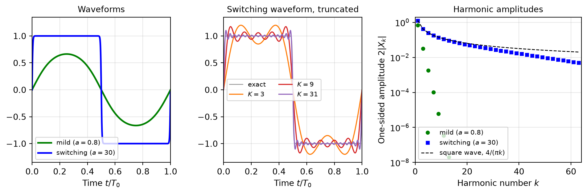
• Sharp edges: many harmonics, ill-conditioning, Gibbs ringing (Figure 108), may not converge, so use PSS
• Convergence: ramp the drive level (source stepping, sweeps)

Harmonic Balance (HB)

Figure 108: Harmonic content of a mildly nonlinear and of a hard-switching waveform, both modeled as \(\tanh(a \sin \omega_0 t)\) (left: \(a = 0.8\) and \(a = 30\)).

Harmonic content of a mildly nonlinear and of a hard-switching waveform, both modeled as \(\tanh(a \sin \omega_0 t)\) (left: \(a = 0.8\) and \(a = 30\)). The harmonics of the mildly nonlinear waveform fall off very quickly, so a few harmonics describe it well. Those of the switching waveform decay only roughly as \(1/k\) (right, one-sided amplitudes \(2|X_k|\)), and a harmonic-balance spectrum truncated at \(K\) harmonics shows Gibbs ringing at the edges (center).

Harmonic Balance (HB)

Table 9: Comparison of shooting (PSS) and harmonic balance (HB)

Property	PSS (shooting)	HB
Domain	time	frequency (devices evaluated in time)
Unknowns	initial state \(\mathbf{x}_0\)	Fourier coefficients \(\mathbf{X}_k\)
Sharp edges, switching	well suited	many harmonics, may not converge
Mildly nonlinear	well suited	very efficient
Distributed elements, S-parameter data	need a time-domain model	exact (simulator-dependent)
Several incommensurate large tones	not possible	well suited
High-Q, long settling	efficient	efficient
Oscillators	autonomous PSS	autonomous HB (simulator-dependent)
Small-signal and noise analyses	PAC, PNOISE	HBAC, HBNOISE

The harmonic count \(K\) is the key accuracy parameter of HB, just as the step size is for a transient analysis. Too small a \(K\) does not show up as a convergence failure: Newton’s method converges, but to the solution of the truncated problem. The convergence in \(K\) need not be monotonic either, so two neighboring values that agree prove little. Compare with a much larger \(K\) or, better, with an independent engine (PSS), and repeat the check over the whole drive sweep, as the required \(K\) grows with the drive level: a value that is sufficient at the nominal level can be several dB off beyond the 1 dB compression point. Oscillators can also be simulated with HB, using an autonomous variant that adds the unknown frequency and a phase condition, similar to the autonomous PSS. Check whether your simulator supports it (in VACASK, oscillators are solved with the autonomous pss).

10.2.4 Periodic Small-Signal Analysis (PAC, HBAC)

\[ \mathbf{G}(t) \, \Delta \mathbf{x}(t) + \frac{\mathrm{d}}{\mathrm{d}t} \left[ \mathbf{C}(t) \, \Delta \mathbf{x}(t) \right] = \Delta \mathbf{u}(t). \tag{80}\]

\[ \sum_{l=-K}^{K} \left[ \mathbf{G}_{k-l} + j (\omega + k \omega_0) \, \mathbf{C}_{k-l} \right] \Delta \mathbf{X}_l = \Delta \mathbf{U}_k, \qquad k = -K, \ldots, K, \tag{81}\]

We now apply a small signal \(\Delta \mathbf{u}(t)\) to a circuit in its periodic steady state \(\mathbf{x}_\mathrm{s}(t)\) and linearize Equation 70 around \(\mathbf{x}_\mathrm{s}(t)\):

In contrast to Equation 72, the Jacobians \(\mathbf{G}(t) = \partial \mathbf{f} / \partial \mathbf{x}\) and \(\mathbf{C}(t) = \partial \mathbf{q} / \partial \mathbf{x}\) are now evaluated along \(\mathbf{x}_\mathrm{s}(t)\) and are periodic in time. The small-signal circuit is a linear periodically time-varying (LPTV) system. Exactly like the time-variant mixer of Section 5.2, such a system converts an input at the offset frequency \(f\) into outputs at all sidebands \(f + k f_0\). We therefore expand the Jacobians into Fourier series, \(\mathbf{G}(t) = \sum_p \mathbf{G}_p e^{j p \omega_0 t}\) (same for \(\mathbf{C}\)), and the excitation and the response into sideband phasors, \(\Delta \mathbf{u}(t) = \sum_k \Delta \mathbf{U}_k e^{j (\omega + k \omega_0) t}\) and \(\Delta \mathbf{x}(t) = \sum_k \Delta \mathbf{X}_k e^{j (\omega + k \omega_0) t}\). Collecting the terms at each sideband yields the conversion matrix equation (Kundert 1999)

which couples the sidebands \(l\) to the sidebands \(k\) through the harmonics \(\mathbf{G}_{k-l}\) and \(\mathbf{C}_{k-l}\) of the time-varying operating point. Without time variation, only \(\mathbf{G}_0\) and \(\mathbf{C}_0\) are nonzero, and Equation 81 falls apart into independent copies of the ac analysis of Equation 72. Solving Equation 81 for a source at sideband \(l\) and observing sideband \(k\) gives the harmonic transfer function \(H_{k,l}(f)\). The offset frequency \(f\) is swept, and each point requires one linear solve of a system with \((2K+1)\) times as many unknowns as the circuit. This is far cheaper than a transient simulation, but the cost grows quickly with \(K\), as discussed below.

Periodic Small-Signal Analysis (PAC, HBAC)

Figure 109: Frequency grid of a periodic small-signal analysis (PAC or HBAC) of a downconversion mixer.

Frequency grid of a periodic small-signal analysis (PAC or HBAC) of a downconversion mixer. The large-signal LO and its harmonics \(k f_\mathrm{LO}\) (gray) are computed by PSS or HB. The small signal lives on the sidebands \(|f + k f_\mathrm{LO}|\) of the swept offset frequency \(f\). The conversion gain is the transfer from the RF input at sideband \(k = +1\) to the IF output at sideband \(k = 0\). The image (\(k = -1\)) and the third-harmonic sidebands (\(k = \pm 3\)) convert to the same IF.

Periodic Small-Signal Analysis (PAC, HBAC)

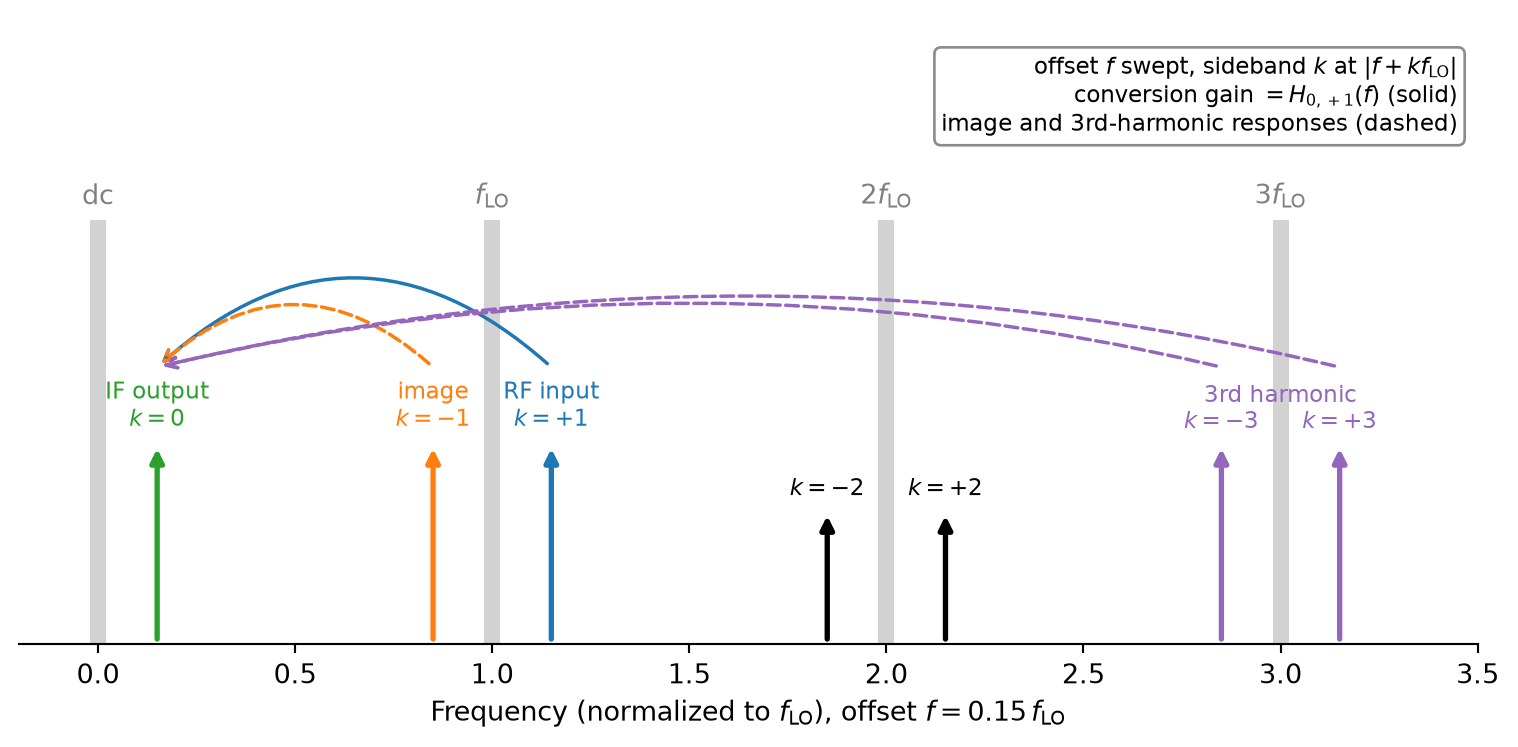
• Conversion gain: \(H_{0,+1}(f)\), RF at \(f_\mathrm{LO} + f\) to IF at \(f\)
• Image response: \(H_{0,-1}(f)\)
• Harmonic responses: \(H_{0,\pm 3}(f)\), interferers around \(3 f_\mathrm{LO}\)
• Upconversion: input at sideband \(0\), output at \(\pm 1\)

Figure 109 shows the frequency grid for a downconversion mixer. The LO is the large signal, the RF and IF are small signals:

• The conversion gain is the transfer from the RF at \(f_\mathrm{LO} + f\) (input sideband \(+1\)) to the IF at \(f\) (output sideband \(0\)), i.e., \(H_{0,+1}(f)\), swept over the IF band in a single analysis.
• The image response is \(H_{0,-1}(f)\) from \(f_\mathrm{LO} - f\). A single mixer converts both sidebands with equal magnitude. In an I/Q (image-reject) receiver, the ratio of the two, evaluated after the I and Q paths are combined, gives the image rejection.
• The harmonic responses \(H_{0,\pm 3}(f)\) show how much of an interferer around \(3 f_\mathrm{LO}\) appears at the IF, which matters for switching mixers in wideband receivers (compare the Fourier series of the switching function in Section 5.2).
• For an upconversion mixer, the input is at the baseband sideband \(0\) and the output at sideband \(\pm 1\).

Periodic Small-Signal Analysis (PAC, HBAC)

Why an AC Analysis of a Mixer Fails

An ac analysis linearizes around the dc operating point, where the LO source sits at its dc value. The mixer is “frozen” in one LO state, the circuit is LTI, and no frequency conversion takes place: the ac analysis shows at most a feedthrough at the RF frequency, but no IF output. Frequency-converting circuits need PAC or HBAC.

Periodic Small-Signal Analysis (PAC, HBAC)

• SC filters, sampling circuits: transfer including aliasing
• N-path filters, passive mixers: input impedance around \(f_\mathrm{LO}\) (Equation 53)
• Power detectors: video response
• Amplifiers under a blocker: desensitization (Equation 11)
• Chopper amplifiers: gain after demodulation, ripple at the chopping harmonics

Further applications of the periodic small-signal analyses are:

• SC filters and sampling circuits, where the clock is the large signal. The transfer from input sideband \(k\) to output sideband \(0\) quantifies aliasing, i.e., how much of an input at \(f + k f_\mathrm{clk}\) appears at \(f\).
• N-path filters and passive mixers, where the input impedance around \(f_\mathrm{LO}\) (see Equation 53) is obtained from the transfer at the same sideband.
• Power detectors, whose video response (the detected baseband output for an amplitude-modulated input) is the transfer from sideband \(\pm 1\) around the carrier to sideband \(0\).
• Amplifiers under a large blocker, where the blocker is the large signal and the wanted signal the small one. This directly shows the gain reduction by desensitization (see Equation 11).
• Chopper amplifiers, where the chopping clock is the large signal. The transfer from input sideband \(0\) to output sideband \(0\) is the gain after demodulation, while the transfers to the sidebands around the chopping harmonics show how much of the signal appears as ripple.

10.2.5 Periodic Noise Analysis (PNOISE, HBNOISE)

1. Modulation. The noise sources depend on the time-varying operating point: channel thermal noise follows the channel conductance (see Section 2.3.1), shot noise follows the current \(I(t)\), and flicker noise depends on the bias as well. Such a source can be written as \(n_i(t) = m_i(t) \, w_i(t)\), with a stationary noise process \(w_i(t)\) and a periodic modulation \(m_i(t)\). Its statistics vary periodically with time, so the noise is cyclostationary.

PAC and HBAC solve the same Equation 81. They differ only in the large-signal solution underneath: PAC builds on the shooting PSS (single fundamental, any waveform shape), HBAC on harmonic balance (also quasi-periodic, e.g., with an LO and a large blocker as two tones, but limited by the harmonic count of the HB solution). The naming follows the engine: the analyses on top of shooting carry a “P” (PAC, PNOISE, and in some simulators PXF and PSP for transfer functions and S-parameters), those on top of harmonic balance carry “HB” (HBAC, HBNOISE, HBXF, HBSP).

The truncation \(K\) of Equation 81 must cover the harmonic content of \(\mathbf{G}(t)\) and \(\mathbf{C}(t)\): a few harmonics are enough for smooth waveforms, while hard-switching circuits like SC filters with steep clock edges can require tens to hundreds of harmonics. For the large signal, the PSS-based analyses have a clear advantage: the periodic steady state is computed in the time domain and is not truncated at all, while HB has to carry all these harmonics in its nonlinear system. In the Gilbert-cell example of VACASK, for instance, a large trapezoidal LO drives the switching quad: HB, and with it HBAC, currently does not converge, while PAC delivers the sidebands with 20 harmonics.

The small-signal step, however, is truncated in both families when it is solved with Equation 81, as in VACASK. Every nonzero Jacobian entry becomes a dense \((2K+1) \times (2K+1)\) block, so the memory grows with \(K^2\). With hard switching, the truncation itself becomes the limit: the truncated Fourier series of a switch conductance does not vanish while the switch is off, so the switch leaks in the small-signal model. On high-impedance nodes, such as the virtual ground of an SC integrator, this spurious leak can falsify the low-frequency gain and noise until \(K\) reaches several hundred, which may be impractical. Check the convergence in \(K\) (keeping in mind that it need not be monotonic, see Section 10.2.3), and fall back to transient simulations where it is not reached.

The noise analysis of Equation 74 misses two effects that a large periodic signal introduces:

Periodic Noise Analysis (PNOISE, HBNOISE)

2. Frequency translation. The LPTV transfer of Equation 81 moves noise from all sidebands \(f + l f_0\) to the output frequency \(f\), which is called noise folding.

Combining both effects, with \(M_{i,m}\) the Fourier coefficients of \(m_i(t)\), \(S_i\) the PSD of the stationary process \(w_i(t)\), and \(H_{i,k}(f)\) the transfer function from source \(i\) at sideband \(k\) to the output, gives the output PSD (Okumura et al. 1993; Roychowdhury et al. 1998)

Periodic Noise Analysis (PNOISE, HBNOISE)

\[ S_\mathrm{out}(f) = \sum_i \sum_{l} \left| \sum_{k} H_{i,k}(f) \, M_{i,k-l} \right|^2 S_i(f + l f_0), \tag{82}\]

with all spectral densities written two-sided. For a constant operating point (\(M_{i,0} = 1\), all other coefficients zero, and \(H_{i,k} = 0\) for \(k \neq 0\)), Equation 82 reduces to Equation 74. A single adjoint solve per offset frequency delivers the transfer functions of all sources, and the results are again broken down into contributions per device and per noise mechanism. PNOISE builds on the shooting PSS, HBNOISE on harmonic balance, exactly as PAC and HBAC. HBNOISE can also start from a multi-tone (quasi-periodic) HB solution, e.g., to obtain the noise figure of a mixer with an LO and a large blocker applied at the same time.

Periodic Noise Analysis (PNOISE, HBNOISE)

Note 10: Noise Folding in an Ideal Switching Mixer

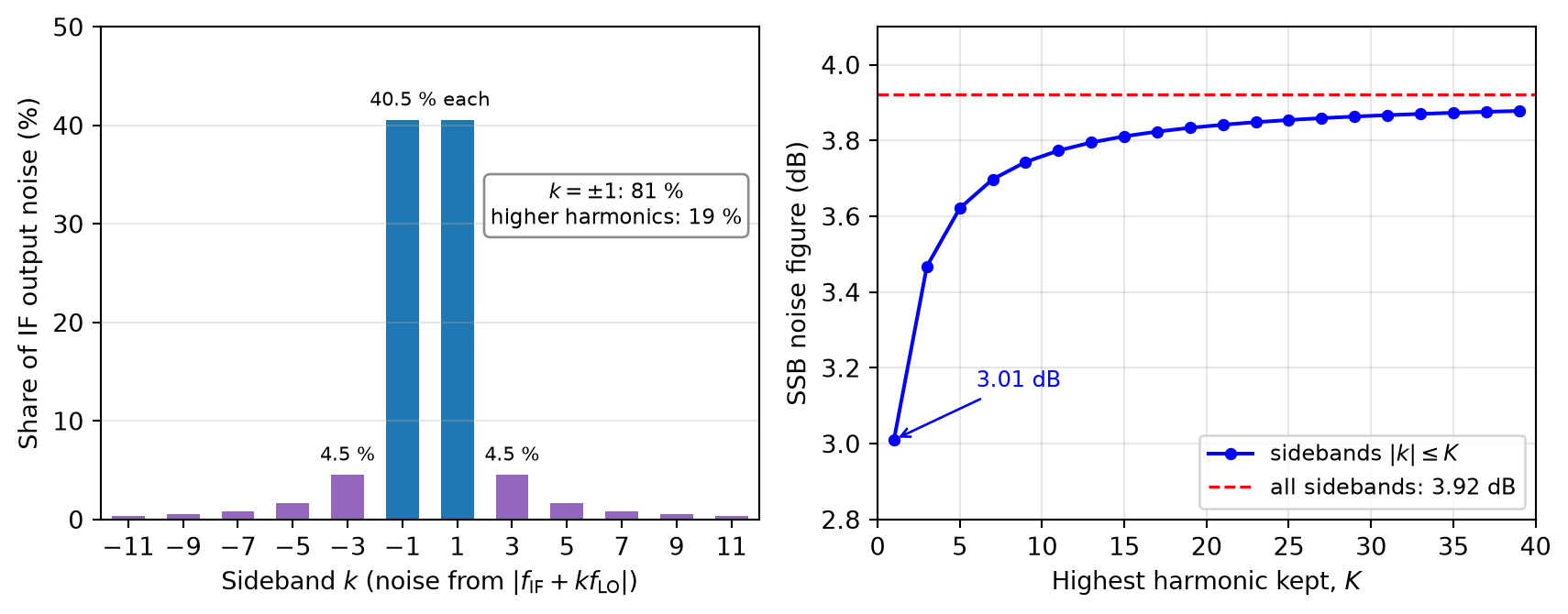
An ideal double-balanced switching mixer multiplies the RF input by a square wave toggling between \(+1\) and \(-1\) with 50% duty cycle (see Section 5.2), whose Fourier coefficients have the magnitude \(|c_k| = 2/(\pi |k|)\) for odd \(k\) and vanish for even \(k\). The switches are noiseless, and the only noise is the white thermal noise of the source resistance, with the PSD \(S_\mathrm{n}\) at every frequency. The noise from each sideband \(k\) folds to the IF with the weight \(|c_k|^2\).

Periodic Noise Analysis (PNOISE, HBNOISE)

Noise Folding in an Ideal Switching Mixer

By Parseval’s theorem, the sum of all weights equals the time average of the squared switching function, which is one:

\[ S_\mathrm{out} = S_\mathrm{n} \sum_{k} |c_k|^2 = S_\mathrm{n}. \]

The wanted RF signal at sideband \(+1\) is converted with the power gain \(|c_1|^2 = 4/\pi^2\). In the single-sideband (SSB) noise factor, only the source noise at the signal frequency counts as input noise, hence

\[ F_\mathrm{SSB} = \frac{S_\mathrm{out}}{|c_1|^2 S_\mathrm{n}} = \frac{\pi^2}{4} \approx 3.9\,\text{dB}. \]

Periodic Noise Analysis (PNOISE, HBNOISE)

Noise Folding in an Ideal Switching Mixer

If the signal occupies both sidebands \(\pm 1\) (as in a direct-conversion receiver), the source noise of both counts as input noise, and the double-sideband (DSB) noise factor is \(F_\mathrm{DSB} = \pi^2/8 \approx 0.9\,\text{dB}\), i.e., 3 dB lower. An analysis that keeps only the sidebands \(\pm 1\) (\(K = 1\)) would miss the 19 % of the noise folded from around \(3 f_\mathrm{LO}\), \(5 f_\mathrm{LO}\), and so on, and underestimate the SSB noise figure by 0.9 dB (3.0 dB instead of 3.9 dB, see Figure 110).

Periodic Noise Analysis (PNOISE, HBNOISE)

Figure 110: Noise folding in an ideal double-balanced switching mixer driven by a square-wave LO with 50 % duty cycle.

Noise folding in an ideal double-balanced switching mixer driven by a square-wave LO with 50 % duty cycle. Left: share of the white source noise that each sideband \(k\) contributes to the IF output, \(|c_k|^2 = (2/(\pi k))^2\) for odd \(k\), and the shares add up to one. Right: single-sideband noise figure obtained when the analysis keeps only the sidebands up to \(|k| \leq K\). Keeping only the first harmonic (\(K = 1\)) underestimates the noise figure by 0.9 dB.

Periodic Noise Analysis (PNOISE, HBNOISE)

• Mixers: SSB/DSB NF incl. image and harmonic folding, LO-translated flicker noise
• Sampling, SC circuits: \(kT/C\) noise from folded wideband noise
• Power detectors: noise with the LO or carrier applied
• Amplifiers under a blocker: blocker noise figure
• Chopper amplifiers: residual flicker noise, white noise folded from the chopping harmonics
• Oscillators: phase noise incl. \(1/f^3\) region from periodic noise (valid down to where numerical errors pin the phase, check the \(1/f^2\) slope) or transient noise, but never from a plain noise analysis

The periodic noise analyses are required wherever a large periodic signal modulates the noise or translates it in frequency:

• Mixers: SSB and DSB noise figure, including the noise folded from the image and from the sidebands of the LO harmonics, and the flicker noise of the switches that the LO translates to the IF (compare the discussion of passive and active mixers in Section 5.2).
• Sampling and SC circuits: wideband switch noise folds into the baseband (\(kT/C\) noise). Many harmonics are needed, and with steep clock edges the conversion matrix may not converge in practice (see Section 10.2.4), so transient noise or an analytic \(kT/C\) budget are the alternatives.
• Power detectors: the noise with the LO (or the input carrier) applied, which can differ substantially from the quiescent noise analysis.
• Amplifiers under a blocker: the noise figure in the presence of a large interferer.
• Chopper amplifiers: the flicker noise that remains at baseband after chopping, and the white noise folded back from the chopping harmonics.
• Oscillators: the phase noise. An oscillator’s noise is cyclostationary by nature, and its noise sources are converted into phase noise in a time-dependent way, which the impulse sensitivity function describes (Hajimiri and Lee 1998). A rigorous nonlinear analysis shows that the phase of an oscillator diffuses like a random walk, so that the output spectrum is a Lorentzian that stays finite at the carrier, whereas a linear analysis predicts phase noise that grows without bound towards the carrier (Demir et al. 2000). RF simulators compute the phase noise with a periodic noise analysis around an autonomous steady state, including the upconverted flicker noise of the \(1/f^3\) region, which Leeson’s equation (Equation 56) does not cover. Such an analysis relies on the time-shift invariance of the oscillator: a time-shifted copy of the periodic solution is a solution, too, so the phase of the linearized circuit is free, and the noise accumulates in it as phase noise that rises with \(1/f^2\) towards the carrier. Every numerical error that breaks this invariance, the harmonic truncation of HB as well as the time discretization of shooting, pins the phase below some offset frequency. A phase noise that flattens towards the carrier instead of rising with \(1/f^2\) is therefore a symptom, not a result, and the analysis has to be refined until this corner lies below the offsets of interest (Note 11). For oscillators with logic-like edges, such as ring oscillators, the periodic noise analysis needs more harmonics than are affordable, and transient noise is the method of choice. A plain noise analysis of an oscillator is meaningless, as it linearizes around the unstable dc operating point.

Periodic Noise Analysis (PNOISE, HBNOISE)

Note 11: Example: Phase Noise of an LC Oscillator in VACASK

A parallel LC tank at \(f_0 = 1\) GHz (\(R_\mathrm{p} = 500\,\Omega\), \(C = 10\) pF, \(Q = 31\)), whose loss is compensated by a noiseless negative conductance \(i = -g_1 v + g_3 v^3\) (Van der Pol), oscillates with \(V_\mathrm{p} = 1\) V. The tank resistance is then the only noise source, and the phase noise follows Equation 57 with \(F = 1\), e.g., \(-126.8\) dBc/Hz at 100 kHz offset. VACASK’s pnoise around the autonomous PSS (pss with oscillator=1) reproduces it within 0.02 dB from 10 kHz to 1 MHz, but only with a fine enough time step.

Periodic Noise Analysis (PNOISE, HBNOISE)

Example: Phase Noise of an LC Oscillator in VACASK

With the default settings, the result flattens below about 20 kHz (\(f_0/50\,000\)) and is already 7.5 dB too low at 10 kHz. The corner depends neither on the number of harmonics (truncharm from 5 to 80 gives the same result) nor on the tolerances, but on the time step with which pnoise integrates the period that it samples for the conversion matrix.

Periodic Noise Analysis (PNOISE, HBNOISE)

Example: Phase Noise of an LC Oscillator in VACASK

Four times as many points per period (pss_minpts) move it four times lower, and limiting the time step between the sampling points (options tran_fbr=0.02 before the pnoise analysis) moved it below 1 kHz, i.e., \(f_0/10^6\). All numbers are from the VACASK version of the IIC-OSIC-TOOLS container 2026.10.

10.3 Choosing the Right Analysis

For the sweep of the offset frequency, keep in mind that the upconverted flicker noise forms narrow skirts around every harmonic of the large signal. A coarse logarithmic sweep easily steps over them, and a point exactly at a harmonic is undefined for \(1/f\) noise. A dense grid near (but not at) the harmonics resolves them.

Choosing the Right Analysis

Table 10: Comparison of the advanced RF analyses

Analysis	Builds on	Linearized	Captures	Main limitation
transient noise	tran	no	in principle everything: switching, folding, jitter, decisions	statistics, run time, numerical artifacts
PSS	shooting (time)	no	periodic steady state, harmonics, oscillation frequency	one common period
HB	Fourier series	no	(quasi-)periodic steady state, IM products	many harmonics for sharp edges
PAC, HBAC	PSS, HB	yes (LPTV)	conversion gain, sideband transfer, aliasing	small signals only
PNOISE, HBNOISE	PSS, HB	yes (LPTV)	cyclostationary noise, folding, mixer NF	small noise only

Table 10 summarizes the advanced analyses, and Figure 111 condenses the selection into two questions: is there a large periodic signal that sets the operating point, and how sharp are the resulting waveforms?

Choosing the Right Analysis

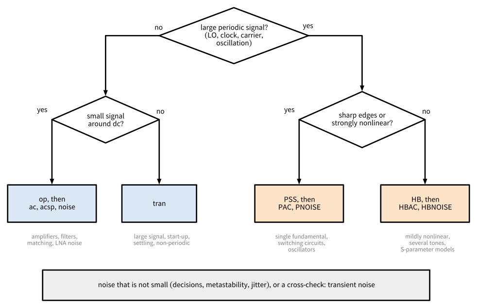
Figure 111: Choosing an analysis.

Choosing an analysis. The first question is whether a large periodic signal (LO, clock, carrier, or the oscillation itself) sets the operating point, the second is how sharp the resulting waveforms are. Transient (noise) simulation remains the reference that every other analysis should be cross-checked against.

Choosing the Right Analysis

Table 11: Recommended analyses for typical RF building blocks.

Circuit	Key metrics	Recommended analyses
LNA	match, gain, NF, stability, \(P_\mathrm{1dB}\), IIP3, blocker NF	op, acsp and noise, HB for \(P_\mathrm{1dB}\) and two-tone IIP3, HBAC and HBNOISE with a blocker
Mixer	conversion gain, SSB/DSB NF, IIP3, image and harmonic rejection	PSS (hard-switching LO) or HB, PAC or HBAC, PNOISE or HBNOISE, two-tone HB for IIP3
Oscillator, VCO	start-up, frequency, tuning range, phase noise	tran for start-up, autonomous PSS, transient noise or periodic noise around the autonomous PSS (simulator-dependent)
SC circuits, sampling, N-path	transfer incl. aliasing, settling, \(kT/C\) noise	tran, PSS, PAC and PNOISE if they converge in \(K\) (not HB), transient noise

For typical RF building blocks, Table 11 lists the key metrics and the recommended analyses. The first analysis in each row is usually the workhorse, and the others refine or cross-check it.

Choosing the Right Analysis

Circuit	Key metrics	Recommended analyses
Power detector	responsivity, compression, video bandwidth, NEP, NF	HB or PSS power sweep, HBAC or PAC, noise with the LO off, HBNOISE or PNOISE with the LO on, transient noise
Power amplifier	output power, efficiency, AM/AM, AM/PM, harmonics	HB power sweep (with EM models of the matching network), PSS for switching PAs, tran
Divider, LO generation	operating range, duty cycle, I/Q phase error, jitter	tran, PSS, PNOISE or transient noise for jitter
Chopper amplifier	gain, ripple, residual flicker noise	tran, PSS with PAC and PNOISE
Comparator, latch	offset, noise, metastability	tran, transient noise

Choosing the Right Analysis

Circuit	Key metrics	Recommended analyses
Passives	Q, S-parameters	acsp with EM-derived models

A complete PLL contains time constants from the VCO period (ns) to the loop settling time (µs), which makes a full transistor-level steady-state simulation very expensive. In practice, the blocks (VCO, divider, phase detector, charge pump) are characterized individually with the analyses above, and the loop is evaluated with the linear phase-domain model of Section 7 and with behavioral transient simulations.

Whatever analysis is used, a result is only trustworthy after it has been checked:

• Convergence parameters. Increase the harmonic count (HB, PAC, PNOISE) well beyond the value that seems sufficient, tighten the maximum time step and the tolerances (tran), and lengthen the stabilization time (PSS) until the result no longer changes, and repeat these checks at the highest drive level.
• Independent methods. HB and PSS compute the same steady state with different algorithms, and where both converge, PAC must agree with HBAC and PNOISE with HBNOISE. PAC or HBAC conversion gain can be compared with a two-tone transient, and PNOISE or HBNOISE with transient noise at reduced noise amplitude. With the large signal switched off, PNOISE and HBNOISE must reproduce the plain noise analysis.
• Simulator messages. A simulation that finishes is not necessarily a correct one. Check the log for aborted analyses, convergence warnings, and devices that were silently dropped from the netlist. Neither a zero exit status nor an existing result file proves that an analysis ran, so delete old results before rerunning.

Choosing the Right Analysis

• Convergence parameters: harmonics, time step, tolerances, stabilization time, also at the highest drive
• Independent methods: HB vs. PSS, PAC vs. HBAC, PNOISE vs. HBNOISE, PAC vs. two-tone tran, PNOISE vs. transient noise, PNOISE without large signal vs. noise
• Simulator messages: a finished run is not a correct one

Choosing the Right Analysis

Note 12: Example: A 160 GHz Power Detector

The open-source SPARX receiver (Dorrer et al. 2026) contains a Schottky-diode power detector at 160 GHz, characterized with VACASK as a mixer with a 159 GHz LO. Its testbenches use most of the analyses of this appendix:

Choosing the Right Analysis

Example: A 160 GHz Power Detector

• HB power sweep for the transfer curve (responsivity and compression), cross-checked with PSS at nine drive levels. The two agree within 1.2 % over an input range of 80 dB.
• HBAC for the conversion gain of each sideband to the IF and the video bandwidth, cross-checked with PAC (within 0.03 dB).

Choosing the Right Analysis

Example: A 160 GHz Power Detector

• noise (LO off) and HBNOISE (LO on) for the noise figure: the LO raises the output noise, so the noise analysis at the dc operating point is 1.2 dB to 2.6 dB optimistic over the IF band, and far more at high LO drive. PNOISE reproduces HBNOISE within 0.2 dB.
• Transient noise with the LO on, run at reduced noise amplitudes and reduced to its linear part, agrees with HBNOISE within about 1 dB.

10.4 Simulator Support

Simulator Support

Table 12: Analyses in the open-source simulators VACASK and ngspice.

Analysis	VACASK (container 2026.10)	ngspice 47
dc operating point, dc sweep	op, op inside a sweep	.op, .dc
ac	ac	.ac
S-parameters	acsp	.sp
noise	noise	.noise
transient	tran	.tran
transient noise	tran with noisefmax (device noise)	.tran with trnoise sources
PSS	pss (driven and autonomous)	.pss (experimental, autonomous only)
HB	hb (single and multi-tone)	not available
PAC, PNOISE	pac, pnoise	not available
HBAC, HBNOISE	hbac, hbnoise	not available

Table 12 lists the analyses of this appendix in the two open-source simulators used in this course, in the ngspice release 47 and the VACASK version of the IIC-OSIC-TOOLS container 2026.10. The ngspice development branch already contains a driven PSS with PAC, PNOISE, PXF and PSP, and quasi-periodic analyses (qpss, qpac, qpnoise), which are not part of a release yet (November 2026). Among the commercial RF simulators, Cadence Spectre RF offers all of them, plus further variants like quasi-periodic shooting and periodic transfer functions and S-parameters (PXF, PSP), while Keysight ADS is built around harmonic balance with its small-signal and noise variants, and adds envelope simulation for modulated signals.

The following VACASK excerpt shows the two-step flow of Section 10.2 for a downconversion mixer: the periodic steady state with the LO is computed and stored once, and the conversion gain and the noise figure are evaluated around it. The RF source carries a unit small-signal excitation at sideband \(+1\), and the IF output (node out) is observed at sideband \(0\). Device models and the mixer itself are omitted, and the syntax is that of the VACASK version above (older builds treated pss as autonomous by default and used other parameter names). The noisy source resistance supplies the input noise. In the pumped circuit, its contribution at the output also contains its noise folded from the image and the harmonic sidebands. The SSB noise factor therefore divides the output noise by the source noise converted from the signal sideband alone, which is \(4 k T R_\mathrm{s}\) times the power gain gain that pnoise reports for the input sideband (as in Note 10), and not by the total contribution of the source resistance.

Simulator Support

// LO: large-signal sine, RF: small-signal tone at sideband +1 (f_LO + f)
vlo (lo 0) vsource type="sine" sinedc=0 ampl=0.5 freq=2.4G
vrf (rfs 0) vsource dc=0 spur={1} smag=[1]
rs (rfs rf) resistor r=50

control
  var flo=2.4G
  analysis op1 op
  // large signal: periodic steady state with the LO, stored for reuse
  analysis pss1 pss tper=1/flo tstab=20/flo store="lo_ss"
  // conversion gain from the RF (sideband +1) to the IF (sideband 0)
  analysis pac1 pac ( ic="lo_ss" psssolve=0 truncharm=40 outharm=0
                      from=100k to=100M mode="dec" points=10 )
  // output noise at the IF, gain from the RF at sideband +1 (SSB NF)
  analysis pn1 pnoise ( ic="lo_ss" psssolve=0 truncharm=40
                        in="vrf" inharm=1 out="out" outharm=0
                        from=100k to=100M mode="dec" points=10 )
endc

The harmonic-balance flow with hb, hbac, and hbnoise is analogous, with three differences: the large signal is described by its fundamental frequencies and harmonic count (e.g., freq=[2.4G] nharm=9) instead of the period, a stored solution is reused with nodeset="lo_ss" hbsolve=0, and spurs are given as tone-weight vectors (e.g., spur={[1]}, outspur=[0], inspur=[1]). VACASK ships worked examples for a Gilbert-cell mixer in multiplier mode (where PAC is compared with HBAC and PNOISE with HBNOISE) and in switching mode (where VACASK’s HB currently does not converge, but PAC and PNOISE do), for the PAC analysis of an SC filter, and for the phase noise of an oscillator from transient noise. Further examples at circuit level, including the 160 GHz power detector, are found in the testbenches of the SPARX repository (Dorrer et al. 2026).

10.5 Summary

Summary

Key Takeaways

• op, ac, acsp, noise linearize around a constant operating point: fast and insightful, but blind to distortion, frequency conversion, and noise folding.
• tran is the general reference, but RF time scales make it expensive, and a maximum time step is mandatory.
• PSS (time domain) and HB (frequency domain) find the periodic steady state directly. PSS suits switching circuits and oscillators, HB mildly nonlinear and multi-tone problems and circuits with distributed elements.

Summary

Key Takeaways

• PAC, HBAC and PNOISE, HBNOISE linearize around this steady state (LPTV) and give conversion gain, aliasing, and cyclostationary noise including folding.
• Transient noise captures everything in principle, at a high cost and with numerical pitfalls. Run at reduced noise amplitude, it is an independent cross-check.
• Increase harmonics, tighten time steps, and compare independent methods before trusting a result.

References

Aprille, T. J., and T. N. Trick. 1972. “Steady-state analysis of nonlinear circuits with periodic inputs.” Proceedings of the IEEE 60 (1): 108–14. https://doi.org/10.1109/PROC.1972.8563.

Bűrmen, Árpád. 2025. VACASK – a novel analog integrated circuit simulator. 60th International Conference on Microelectronics, Devices and Materials (MIDEM 2025), Ljubljana, Slovenia. https://doi.org/10.5281/zenodo.17434615.

Demir, A., A. Mehrotra, and J. Roychowdhury. 2000. “Phase noise in oscillators: a unifying theory and numerical methods for characterization.” IEEE Transactions on Circuits and Systems I: Fundamental Theory and Applications 47 (5): 655–74. https://doi.org/10.1109/81.847872.

Dorrer, Simon, David Kellerer-Pirklbauer, and Harald Pretl. 2026. GitHub Repository for SPARX: An Open-Source, Automated, Programmatically Generated, Frequency-Scalable Six-Port Receiver in 130-nm CMOS. https://doi.org/10.5281/zenodo.19654232.

Hajimiri, A., and T. H. Lee. 1998. “A general theory of phase noise in electrical oscillators.” IEEE Journal of Solid-State Circuits 33 (2): 179–94. https://doi.org/10.1109/4.658619.

Kundert, K. S. 1999. “Introduction to RF simulation and its application.” IEEE Journal of Solid-State Circuits 34 (9): 1298–319. https://doi.org/10.1109/4.782091.

Nagel, Laurence W. 1975. SPICE2: A Computer Program to Simulate Semiconductor Circuits. Memorandum ERL-M520. Electronics Research Laboratory, University of California, Berkeley.

Nakhla, M., and J. Vlach. 1976. “A piecewise harmonic balance technique for determination of periodic response of nonlinear systems.” IEEE Transactions on Circuits and Systems 23 (2): 85–91. https://doi.org/10.1109/TCS.1976.1084181.

Okumura, M., H. Tanimoto, T. Itakura, and T. Sugawara. 1993. “Numerical noise analysis for nonlinear circuits with a periodic large signal excitation including cyclostationary noise sources.” IEEE Transactions on Circuits and Systems I: Fundamental Theory and Applications 40 (9): 581–90. https://doi.org/10.1109/81.244907.

Pozar, David M. 2011. Microwave Engineering. 4th edition. Wiley.

Razavi, Behzad. 2020. “The Design of a Comparator [The Analog Mind].” IEEE Solid-State Circuits Magazine 12 (4): 8–14. https://doi.org/10.1109/MSSC.2020.3021865.

Roychowdhury, J., D. Long, and P. Feldmann. 1998. “Cyclostationary noise analysis of large RF circuits with multitone excitations.” IEEE Journal of Solid-State Circuits 33 (3): 324–36. https://doi.org/10.1109/4.661198.

Telichevesky, Ricardo, Kenneth S. Kundert, and Jacob K. White. 1995. “Efficient steady-state analysis based on matrix-free Krylov-subspace methods.” Proceedings of the 32nd ACM/IEEE Design Automation Conference (DAC), 480–84. https://doi.org/10.1145/217474.217574.

References