Transceivers

Radio-Frequency Integrated Circuits

3 Transceivers

3.1 Direct-Conversion Transceiver

Nowadays, the various small-signal RF functions for receive and transmit are integrated into so-called transceivers (TRX). A TRX is a device that can both transmit and receive signals, and is usually called an “RFIC”. While high monolithic integration is certainly the norm for radio-frequency devices intended for standards like Bluetooth, Wi-Fi, cellular, etc., it is increasingly used also for mm-wave frequencies for applications like automotive radar and 5G cellular.

Typically, TRX include components like amplifiers, mixers, filters, oscillators, and phase-locked loops. When digital interfaces are used for the baseband I/Q data, also functions like analog-to-digital conversion (ADC) and digital-to-analog conversion (DAC) are integrated together with digital signal processing (DSP) blocks and potentially high-speed interfaces (because for wide bandwidths the I/Q sample rate can get quite high).

In these notes we will focus on the RF part of the TRX, which is responsible for the upconversion of baseband or intermediate frequency (IF) signals to the desired transmit frequency during transmission, and the downconversion of received signals from the carrier frequency to baseband or IF during reception. For filters, low-frequency amplifiers, ADCs, DACs, and DSP blocks we refer to related courses and literature, for example our analog circuit design course.

Direct-Conversion Transceiver

• Pulse shaping of the baseband signal (mostly digital)
• Up-/downconversion to/from the carrier frequency
• Contain the TX signal in a small bandwidth; single out the wanted RX signal with adequate SNR
• Adapt gain (and linearity) to the RX signal and TX output power
• Generate the LO with low phase noise

The following typical functions have to be performed by a TRX:

• Pulse-shaping filtering of the baseband signal (which can be implemented in analog or, in most cases, digital form).
• Modulating the baseband signal onto a carrier frequency (upconversion) in the TX or downconversion in the RX.
• Contain the RF signal in a small bandwidth (TX), or single out the wanted signal in the RX with adequate signal to noise ratio (SNR).
• Adapt gain (and linearity) to the signal strength in the RX, and to the output power in the TX.
• Generate the carrier frequency (local oscillator, LO) with low phase noise.

Direct-Conversion Transceiver

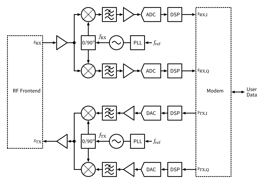
Figure 19: Block diagram of a typical transceiver (TRX) showing the main functional blocks of RX and TX.

The dominant architecture for the TRX is the so-called direct-conversion or zero-IF architecture, where the up- and downconversion are performed in a single step (Razavi 2011). This is in contrast to super-heterodyne architectures, where the signal is first converted to an intermediate frequency (IF) before being converted to baseband. The direct-conversion architecture has the advantage of reduced complexity and cost, as it requires fewer components and less filtering. However, it also has some disadvantages, such as increased susceptibility to dc offsets and I/Q imbalance. A typical TRX block diagram is shown in Figure 19.

Block diagram of a typical transceiver (TRX) showing the main functional blocks of RX and TX. The modem provides the digital baseband processing and interfaces to the rest of the system. For implementation options of the RF front-end, see Section 3.5.

3.2 Modulation and Demodulation

As can be seen in Figure 19, this generic architecture can be adapted in various ways. Generally, the amplifier gains are adjustable to adapt to different signal levels. If adaptive channel bandwidths are to be supported, the corner frequencies of the low-pass filters (LPF) can be adjusted, as well as (optionally) the sampling rate of the ADCs and DACs. The local oscillator (LO) frequency is generated by a phase-locked loop (PLL) synthesizer, which can be tuned to the desired carrier frequency. In case of frequency-division duplex (FDD) operation, two PLLs are used to generate the TX and RX LO frequencies, which are separated by the duplex distance \(f_\mathrm{dpx}\). In time-division duplex (TDD) operation, a single PLL is sufficient, supplying the LO signal to both RX and TX.

The modem (short for modulator-demodulator) that is shown in Figure 19 is responsible for the digital baseband processing, including functions like channel coding/decoding, modulation/demodulation, equalization, error correction, encryption/decryption, and framing/timing. The modem is usually implemented as a digital System-on-Chip (SoC) consisting of (multiple) CPUs, DSPs, and fixed-function blocks for time-critical processing. For an in-depth discussion we recommend (Sklar and Harris 2020) or (Molisch 2022).

Modulation and Demodulation

\[ \tilde{s}_\mathrm{BB}(t) = s_\mathrm{I}(t) + j \cdot s_\mathrm{Q}(t). \]

\[ \tilde{s}_\mathrm{RF}(t) = \tilde{s}_\mathrm{BB}(t) \cdot e^{j \omega_\mathrm{c} t} = [s_\mathrm{I}(t) + j \cdot s_\mathrm{Q}(t)] \cdot [\cos(\omega_\mathrm{c} t) + j \cdot \sin(\omega_\mathrm{c} t)]. \]

Modulation is the process of varying a carrier signal at frequency \(f_\mathrm{c}\) in order to transmit information. The complex baseband signal (after converting the real-valued in-phase and quadrature signals \(s_\mathrm{I}\) and \(s_\mathrm{Q}\), respectively, to analog and applying pulse-shaping filtering) is represented as (\(\tilde{s}_\mathrm{BB} \in \mathbb{C}\); \(s_\mathrm{I}, s_\mathrm{Q} \in \mathbb{R}\)) (Martin 2004):

We want to shift this signal to the carrier frequency \(f_\mathrm{c}\) to create the modulated RF signal \(\tilde{s}_\mathrm{RF} \in \mathbb{C}\), which can be done by multiplying with a complex exponential (\(e^{j \omega_\mathrm{c} t}\), with \(\omega_\mathrm{c} = 2 \pi f_\mathrm{c}\)):

The real-valued RF signal \(s_\mathrm{RF} \in \mathbb{R}\) is obtained from \(\tilde{s}_\mathrm{RF}\) by complex-conjugate symmetry

Modulation and Demodulation

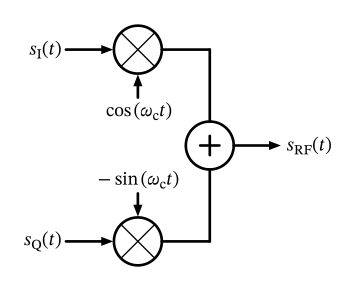
\[ s_\mathrm{RF}(t) = \frac{1}{2} \left[ \tilde{s}_\mathrm{RF}(t) + \tilde{s}_\mathrm{RF}^*(t) \right] = s_\mathrm{I}(t) \cos(\omega_\mathrm{c} t) - s_\mathrm{Q}(t) \sin(\omega_\mathrm{c} t). \tag{27}\]

The process formulated in Equation 27 is done in hardware in the TX modulator, as shown in Figure 20.

Modulation and Demodulation

Figure 20: TX modulator.

Modulation and Demodulation

\[ \begin{split} s_\mathrm{RF}(t) &= \frac{1}{2} \left[ A(t) \cdot e^{j \omega_\mathrm{c} t + j \varphi(t)} + A(t) \cdot e^{-j \omega_\mathrm{c} t -j \varphi(t)} \right]\\ &= A(t) \cdot \cos[ \omega_\mathrm{c} t + \varphi(t) ] \end{split} \]

The RF signal generation according to Equation 27 is called quadrature modulation. This is the modulation method used most often in modern (broadband) communication systems, as it allows one to transmit two independent signals (I and Q) in the same bandwidth. The I and Q signals are also called quadrature components, as they are 90° out of phase with each other.

Alternatively, a modulation method called polar modulation can be used, where the amplitude and phase of the carrier are varied according to (again using the complex-conjugate symmetry to obtain a real-valued signal):

This is done by converting the baseband I and Q signals (\(s_\mathrm{I}\) and \(s_\mathrm{Q}\)) to polar coordinates with

Modulation and Demodulation

\[ A(t) = \sqrt{s_\mathrm{I}^2(t) + s_\mathrm{Q}^2(t)}, \quad \varphi(t) = \tan^{-1} \left[ \frac{s_\mathrm{Q}(t)}{s_\mathrm{I}(t)} \right]. \]

As the mathematical operations required for the Cartesian to polar transformation are quite nonlinear, the \(A(t)\) and \(\varphi(t)\) signals are wideband. While fairly complex to implement, polar modulation can have an efficiency advantage in the TX circuits, as the signal loss associated with quadrature combination can be avoided (Fulde et al. 2017).

For narrowband wireless standards the use of polar modulation can be quite efficient, as for example Bluetooth, where basically all transmitters are realized as polar modulators.

In the RX, the received RF signal is downconverted to baseband by the inverse process of Figure 20, shown in Figure 21.

Modulation and Demodulation

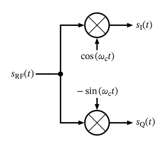
Figure 21: RX demodulator.

Modulation and Demodulation

\[ \begin{split} \tilde{s}_\mathrm{BB}(t) &= s_\mathrm{RF}(t) \cdot e^{-j \omega_\mathrm{c} t}\\ &= s_\mathrm{RF}(t) \cdot [\cos(\omega_\mathrm{c} t) - j \cdot \sin(\omega_\mathrm{c} t)]\\ &\overset{\text{LPF}}{=} \frac{1}{2} \left[ s_\mathrm{I}(t) + j \cdot s_\mathrm{Q}(t) \right]. \end{split} \tag{28}\]

For demodulation we have to shift the RF signal down to baseband, which mathematically is done by multiplying with the negative complex carrier frequency \(e^{-j \omega_\mathrm{c} t}\)

In hardware this is realized with two mixers, producing \(s_\mathrm{RF}(t) \cdot \cos(\omega_\mathrm{c}t)\) in the I path and \(-s_\mathrm{RF}(t) \cdot \sin(\omega_\mathrm{c}t)\) in the Q path. Each of these products contains, besides the wanted baseband term, a component at \(2 \omega_\mathrm{c}\), which is why Equation 28 only holds after the subsequent low-pass filter (indicated by the “LPF” above the equal sign). The factor of one-half that the recovered baseband signals carry is of no consequence, as it is simply absorbed by the RX gain.

3.3 Filtering

Filtering

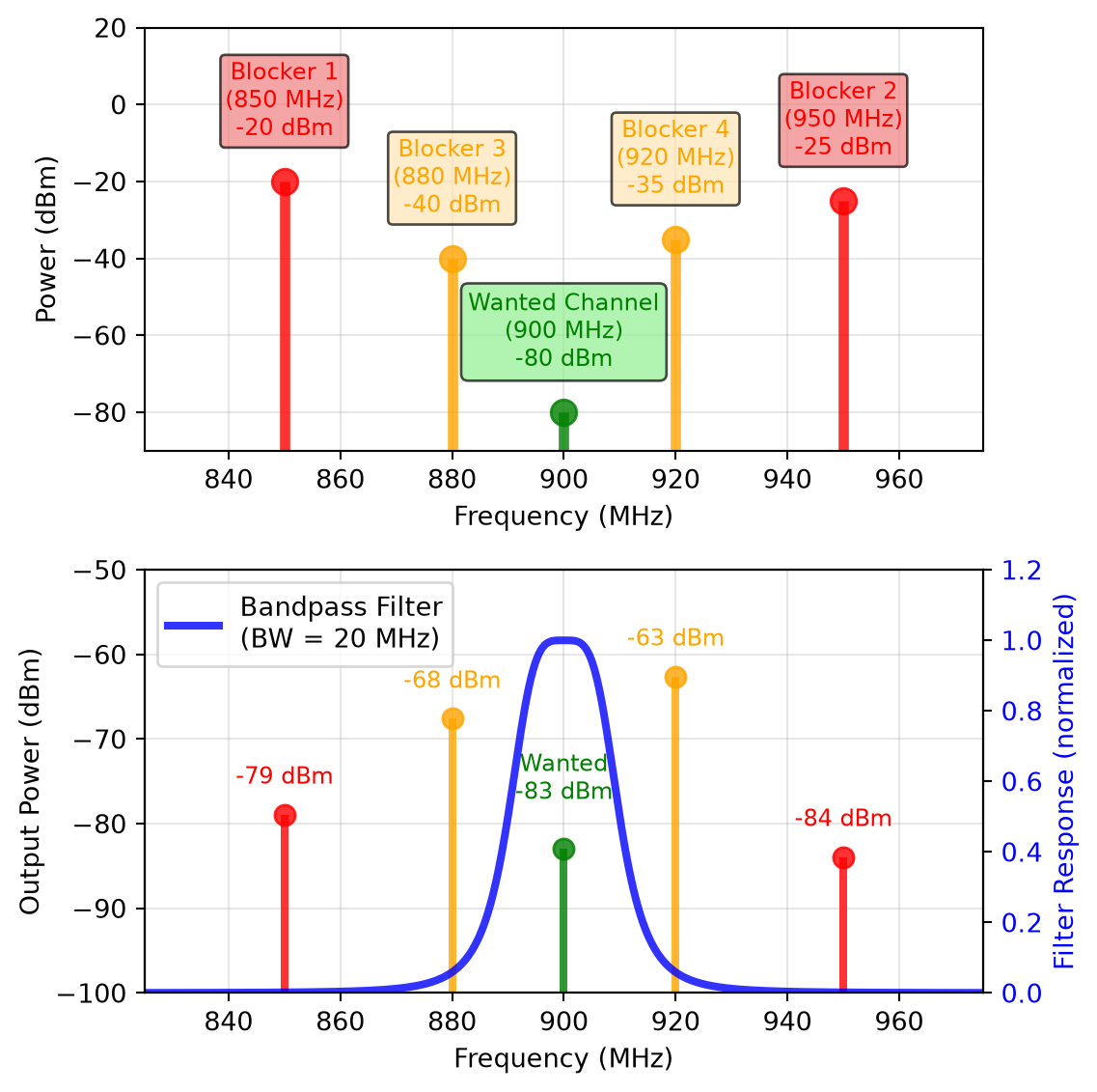
Figure 22: Filtering of wanted channel amid strong unwanted blockers.

Filtering is an essential function in both TX and RX. In the TX, filtering is used to limit the bandwidth of the transmitted signal to the allocated channel bandwidth, and to suppress out-of-band emissions. In the RX, filtering is used to select the wanted signal from a crowded spectrum, and to suppress unwanted signals (blockers) that can cause interference or desensitization of the RX.

A typical example of filtering in the RX is shown in Figure 22, where a bandpass filter is used to attenuate strong unwanted blockers while only slightly attenuating the wanted signal.

Filtering of wanted channel amid strong unwanted blockers. An exemplary RX scenario around 900 MHz is shown: The strong blockers (top figure) are attenuated by an RF bandpass filter (bottom figure) with a bandwidth of 20 MHz, achieving more than 40 dB rejection of the blockers while only slightly attenuating the wanted signal.

Filtering

\[ Q = \frac{f_\mathrm{c}}{\Delta f} \]

In any filter there exists a fundamental trade-off between selectivity (steepness of the filter skirts), bandwidth, and insertion loss. A very selective filter with steep skirts and large passband BW will have a high insertion loss. Conversely, a filter with low insertion loss will have a gentle roll-off and may not sufficiently suppress unwanted signals.

A useful metric to quantify the performance of a filter is the quality factor \(Q\), defined as

where \(f_\mathrm{c}\) is the center frequency and \(\Delta f\) is the \(-3\) dB bandwidth of the filter. A high \(Q\) indicates a narrow-band filter.

The achievable \(Q\) depends on the used filter technology. For example, on-chip \(LC\) filters can achieve \(Q\) values of around 10–20, while off-chip SAW or BAW/FBAR filters reach \(Q\) values into the thousands, and a crystal filter can achieve \(Q\) values of several tens of thousands.

The choice of filter technology depends on the application requirements, such as frequency range, bandwidth, insertion loss, cost, and power handling. Generally speaking, the required filtering to single out the wanted signal in the RX spectrum and decrease the power of strong blockers to a tolerable level is one of the most critical design choices, and is usually distributed at different locations in the RX chain:

• RF filters (between antenna and LNA) provide a first level of filtering, and are usually implemented as off-chip SAW or BAW/FBAR filters. They provide high \(Q\) and good selectivity, but have a fixed center frequency and bandwidth. They are used to pass the wanted band of interest, and to attenuate strong out-of-band blockers.
• IF filters (in case of a super-heterodyne receiver) provide additional filtering, and can be implemented as on-chip LC filters or off-chip SAW/BAW filters. They provide moderate \(Q\) and selectivity, and can be tuned to some extent.
• BB filters (after downconversion) provide the final level of filtering before entering the ADCs, and are usually implemented as on-chip active \(RC\) filters. They provide channel selection, and can be easily adjusted to different bandwidths.
• Digital filters (in the DSP block) provide the final level of filtering and signal processing, and can be implemented as FIR or IIR filters. They provide high flexibility and can be easily adapted to different standards and requirements. Digital filters show no variations, so they can be designed to be very selective.

Filtering

• RF filters (antenna to LNA): off-chip SAW or BAW/FBAR, high \(Q\), fixed; pass the band, attenuate out-of-band blockers
• IF filters (super-heterodyne): on-chip \(LC\) or off-chip SAW/BAW, moderate \(Q\)
• BB filters: on-chip active \(RC\), channel selection, adjustable bandwidth
• Digital filters (FIR/IIR): flexible, no variations, very selective

Filtering

Filter Technologies Primer

Technology	\(Q\)	Remarks
Active \(RC\), \(g_\mathrm{m}C\) (on-chip)	low	Tunable baseband filters (Schaumann et al. 2009; Zverev 1967)
Digital FIR/IIR	n/a	Programmable, no variations; power/area vs. performance
\(LC\) on-chip / off-chip	10–20 / 50–100	Tunable via \(C\) (easy) or \(L\) (difficult)
Ceramic (off-chip)	up to hundreds	Smaller and cheaper than SAW/BAW
SAW, BAW/FBAR (off-chip)	thousands	Fixed; 1–2 filters per band
Waveguide	thousands	Above 10 GHz; bulky, base stations
Crystal	tens of thousands	Bulky, expensive, up to tens of MHz
Optical	extremely high	Requires electrical-optical conversion

It is important to note (because this dictates a lot of choices in RF design) that high-\(Q\) filters are usually fixed-frequency and fixed-bandwidth. Only baseband and digital filters can be easily adjusted to different bandwidths!

Baseband filters (analog) are usually implemented as active \(RC\) filters on-chip (Schaumann et al. 2009; Zverev 1967). They are very flexible and can have adjustable bandwidth by changing \(R\) and/or \(C\). For medium/high frequencies \(g_\mathrm{m}C\) filters can be used, which are also tunable by changing the transconductance \(g_\mathrm{m}\) and/or \(C\). For even higher bandwidths, on-chip LC filters can be used, which have a limited \(Q\) of around 10–20.

Baseband filters (digital) are implemented as FIR or IIR filters. They can be made programmable and can be easily adapted to different requirements. Digital filters show no variations, so they can be designed to be very high performance. However, a trade-off between power consumption/area (number of bits and operations) and performance exists.

Surface acoustic wave (SAW) and bulk acoustic wave (BAW/FBAR) filters are specialized off-chip components that can achieve high \(Q\) into the thousands. They have a fixed center frequency and bandwidth. Usually 1–2 such filters are required per supported band of interest, which can drive up implementation cost and PCB area for RF front-ends that shall support many different frequency bands.

Crystal filters can achieve very high \(Q\) values of several tens of thousands, but are usually bulky and expensive and limited to an operating frequency of tens of MHz.

LC filters can be either implemented off-chip (using discrete components) or on-chip. Off-chip \(LC\) filters can achieve higher \(Q\) values than on-chip \(LC\) filters, but are usually larger and more expensive. On-chip \(LC\) filters are limited in \(Q\) (around 10–20), but are very compact and can be integrated into the RFIC. Off-chip \(LC\) filters can achieve \(Q\) values of around 50–100, depending on the frequency and component quality. \(LC\) filters can be made tunable by changing \(L\) (difficult) and/or \(C\) (easy).

Ceramic filters are another off-chip filter technology that can achieve moderate to high \(Q\) values (up to several hundreds). They are usually smaller and less expensive than SAW or BAW/FBAR filters, but also have lower performance.

Waveguide filters are used at very high frequencies (above 10 GHz) and can achieve very high \(Q\) values (up to several thousands). They are usually bulky and expensive, and are not commonly used in mobile applications, but rather in fixed installations like base stations or satellite communication.

Optical filters can have extremely high \(Q\) values but are difficult to apply in electronic RF systems due to the need for optical components and the challenge of integrating them with electronic circuits, as well as the required electrical-optical signal conversion.

3.4 Direct-Conversion Architecture

Fundamentally, the choice of filter technology is a trade-off between performance, size, cost, power handling, and flexibility. In most cases, a combination of different filter technologies is used to achieve the desired performance.

Direct-Conversion Architecture

• A single LO per RX/TX chain (shared in TDD)
• Minimum number of RF blocks: low cost and power
• Flexible, even wideband, with very good performance
• High integration level: almost everything on-chip
• De facto standard for cellular, Wi-Fi, Bluetooth (RX), and GNSS

The transceiver architecture shown in Figure 19 is called the direct-conversion or zero-IF architecture, as the downconversion in the RX and upconversion in the TX are done in a single step. This architecture has several advantages:

• Per RX- and TX-chain a single LO is required (which can even be shared between RX and TX in TDD operation).
• There are a minimum number of RF blocks, which is good for cost and power consumption.
• This architecture is very flexible and can be easily adapted to different standards and requirements, even for wideband operation. It generally shows very good performance if the disadvantages can be overcome by good design.
• This architecture allows a high integration level, as basically all blocks can be implemented on-chip.
• Direct conversion is the de facto standard architecture for cellular, Wi-Fi, Bluetooth (with the exception of the TX), and GNSS.

Direct-Conversion Architecture

• LO-RF coupling: self-mixing and RX desensitization, TX LO leakage
• Low IIP2: desensitization by AM blockers (Gebhard et al. 2019)
• TX LO pulling (LO and RF at the same frequency)
• I/Q errors: constellation distortion, increased EVM
• dc offsets from LO self-mixing and IM2
• Flicker noise: TX close-in noise, RX noise figure

However, the direct-conversion architecture also has some serious disadvantages:

• LO-RF coupling can cause self-mixing and desensitization of the RX, as well as LO leakage in the TX. This is an issue because the LO frequency is the same as the RF carrier frequency.
• Even-order distortion (characterized by a low IIP2) causes sensitivity degradation due to strong amplitude-modulated blockers (Gebhard et al. 2019).
• LO pulling can occur in the TX (as, again, LO and RF are at the same frequency).
• I/Q errors (amplitude and phase mismatch) of the \(I\) and \(Q\) paths can cause constellation distortion leading to increased error vector magnitude (EVM).
• Significant dc offsets can occur due to self-mixing of LO leakage or the even-order distortion products (IM2).
• Flicker noise (1/f noise) upconversion can cause increased TX noise close to the carrier, as well as increased RX noise figure.

3.5 Duplexing

Nowadays there exist good design techniques to mitigate these disadvantages. However, in some cases (for example very high linearity requirements, or very high frequencies) other architectures like low-IF or super-heterodyne may be preferable.

3.5.1 Frequency-Division Duplex (FDD)

In the block diagram of Figure 19, we have not yet considered how to share a single antenna between RX and TX. Essentially, there are two main methods to achieve this: frequency-division duplex (FDD) and time-division duplex (TDD).

A special case beyond FDD and TDD is full-duplex (FD), where RX and TX operate simultaneously in the same frequency band. Full-duplex is technically challenging, as it requires very high isolation between RX and TX, which is difficult to achieve in practice. For some special applications, like radar, full-duplex operation is possible, but for most communication systems FDD or TDD is used.

In FDD, the RX and TX operate at different frequencies, separated by a duplex distance \(f_\mathrm{dpx} = | f_\mathrm{RX} - f_\mathrm{TX} |\). This allows simultaneous transmission and reception, which is beneficial for applications like voice communication where low latency is required. However, FDD requires two separate frequency bands, which can be a limitation in terms of spectrum availability. Additionally, FDD requires two PLLs to generate the RX and TX LO frequencies, which increases complexity and power consumption.

The RF RX and TX paths are connected to the antenna via a duplexer filter, which is a three-port device that allows signals to pass between the antenna and the RX or TX path, while isolating the RX and TX paths from each other. A typical FDD TRX block diagram is shown in Figure 23.

Frequency-Division Duplex (FDD)

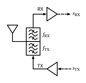
Figure 23: Block diagram of an FDD RF front-end.

Frequency-Division Duplex (FDD)

• RX and TX can operate simultaneously, which is beneficial for low-latency applications.
• There is no need for fast switching between RX and TX, which simplifies the timing control.
• FDD allows relaxed synchronization requirements between RX and TX and different users.

Advantages of FDD:

Disadvantages of FDD:

• Duplexer filters are costly components with significant insertion loss depending on filtering requirements.
• It requires two separate frequency bands, which can be a limitation in terms of spectrum availability and MIMO channel estimation.
• The strong TX leakage via the duplexer filter into the RX path causes severe desensitization of the RX, which requires high linearity and good filtering (50 dB to 60 dB).
• The RX and TX chains (including their PLLs) are operating simultaneously, which increases power consumption and can cause interference between the RX and TX paths (e.g., LO pulling).

Frequency-Division Duplex (FDD)

• Duplexers are costly and add insertion loss
• Two separate frequency bands needed (spectrum, MIMO channel estimation)
• TX leakage desensitizes the RX: high linearity and 50 dB to 60 dB filtering needed
• RX and TX run simultaneously: higher power, RX/TX interference (LO pulling)

3.5.2 Time-Division Duplex (TDD)

In TDD, the RX and TX share the same frequency band but operate at different times. This allows for more efficient use of the available spectrum, as the same channel frequency can be used for both transmission and reception. TDD is particularly well-suited for applications with asymmetric traffic patterns, where the data rate in one direction is significantly higher than in the other. However, TDD requires precise timing control to avoid interference between RX and TX periods, which can increase complexity.

In TDD, a single PLL can be used to generate the LO frequency for both RX and TX, which reduces complexity and power consumption. The RX and TX RF paths are connected to the antenna via a switch, which alternates between connecting the antenna to the RX path and the TX path. A typical TDD TRX block diagram is shown in Figure 24.

Time-Division Duplex (TDD)

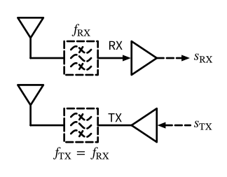
Figure 24: Block diagram of a TDD RF front-end.

Time-Division Duplex (TDD)

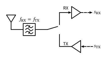
• More efficient use of the available spectrum, as the same frequency can be used for both RX and TX.
• A single PLL can be used for both RX and TX, which reduces complexity and power consumption.
• No duplexer is required (just a single band filter), which reduces cost and insertion loss.
• No RX blocking by own TX, which relaxes linearity and filtering requirements.
• MIMO is easier to implement, as all antennas can operate in the same frequency band.

Advantages of TDD:

Disadvantages of TDD:

Time-Division Duplex (TDD)

• RX and TX cannot operate simultaneously, which can be a limitation for low-latency applications.
• TDD requires precise timing control to avoid interference between RX and TX periods, which can increase complexity.
• Synchronization between RX and TX and different users is required, which can be challenging in some scenarios.

3.5.3 Comparison of FDD and TDD

Table 4: Comparison of duplexing methods used by major wireless standards

Wireless Standard	Duplexing Method	Comments
GSM (2G)	FDD & TDMA	TX and RX operate at different frequencies (FDD) and different times (TDMA)
UMTS (3G)	FDD	Traditional cellular standard using paired spectrum
LTE (4G)	FDD/TDD	FDD is used mostly <2.7 GHz, TDD is used >2.3 GHz
5G NR	FDD/TDD	FDD is used mostly <2.7 GHz, TDD is used >2.3 GHz
Wi-Fi (802.11)	TDD	Unlicensed spectrum operation
Bluetooth	TDD	Short-range personal area network
Zigbee	TDD	Low-power IoT applications

Below is a summary of important wireless standards and their duplexing method as shown in Table 4.

As you can see in Table 4, there is a tendency to use FDD for lower frequencies and long communication distances, while TDD is preferred for higher frequencies and shorter distances.

3.5.4 Full Duplex (FD)

In case of FD, neither a duplexer nor a switch can be used in the RF front-end. One popular method (which also helps to increase the RX-TX isolation) is to use two antennas, as shown in Figure 25. The TX antenna is used to transmit the signal, while the RX antenna is used to receive the signal. The two antennas are placed in such a way that they are isolated from each other, which helps to reduce the interference between the RX and TX paths. Also polarization diversity can be used to further increase the isolation.

Full Duplex (FD)

Figure 25: Block diagram of an in-band full-duplex (FD) RF front-end using two separate antennas for RX and TX, which operate simultaneously at the same frequency.

Full Duplex (FD)

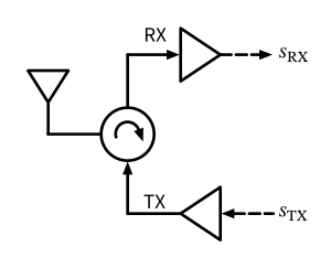
Figure 26: Block diagram of an in-band full-duplex (FD) RF front-end using a single antenna and a circulator.

Another method to achieve FD operation is to use a circulator, which is a three-port device that allows signals to flow in one direction while isolating the other two ports. The circulator can be used to connect the RX and TX paths to the same antenna, while providing isolation between them. A typical FD TRX block diagram using a circulator is shown in Figure 26.

Block diagram of an in-band full-duplex (FD) RF front-end using a single antenna and a circulator. The circulator routes TX to the antenna and the antenna to RX, while isolating the TX from the RX port.

3.6 Specialty Architectures

Regardless of whether two antennas or a circulator are used, the isolation between the TX and RX paths is always finite (typically only in the range of 15 dB to 20 dB for a circulator). As a consequence, a large fraction of the own (and strong) TX signal leaks directly into the sensitive RX port. Practical FD systems therefore require additional self-interference cancellation (also called leakage cancellation), performed in the RF/analog and/or digital domain, to suppress this residual TX leakage below the RX noise floor (Sadjina et al. 2020).

3.6.1 Super-Heterodyne Architecture

In some cases, other architectures may be preferred over the direct-conversion architecture. During the evolution of wireless communication, many different architectures have been proposed and used. However, only a few of them are still relevant today. A few examples are shown next.

The super-heterodyne architecture is a widely used approach in radio. It works by mixing the incoming/outgoing RF signal with an LO to produce an intermediate frequency (IF) signal. This IF signal is then amplified and processed, allowing for better selectivity and sensitivity compared to direct-conversion architectures. Super-heterodyne receivers and transmitters are known for their excellent performance in terms of image rejection and dynamic range, making them suitable for a variety of applications, including traditional analog TV and radio broadcasting. A simplified block diagram of a super-heterodyne transceiver is shown in Figure 27.

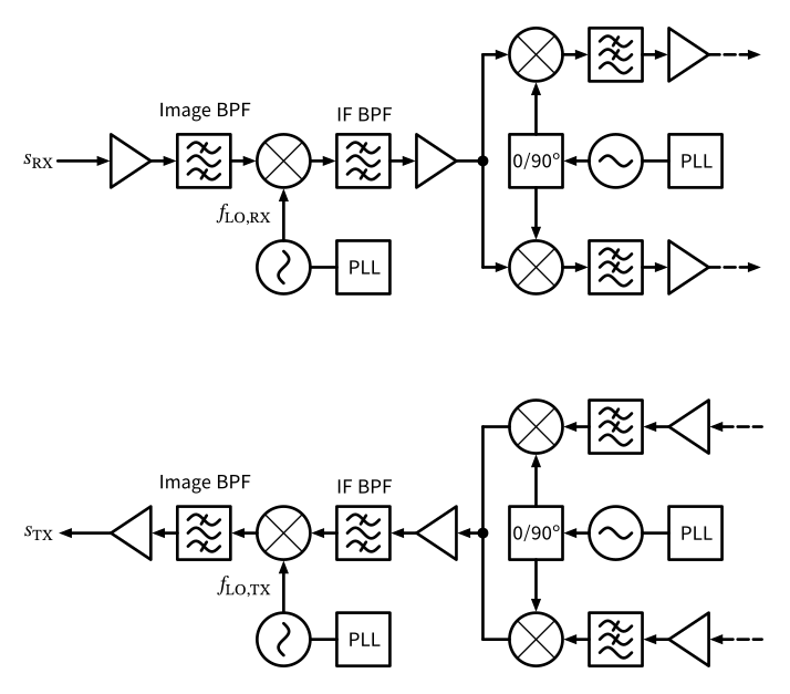
Super-Heterodyne Architecture

Figure 27: Block diagram of a super-heterodyne transceiver (TRX) showing the main functional blocks of RX and TX.

3.6.2 Low-IF Architecture

When you compare Figure 19 with Figure 27, you can immediately appreciate the increased complexity of the super-heterodyne architecture. It requires two PLLs to generate the RX and TX LO frequencies, as well as additional mixers, amplifiers, and filters for the IF stage. This increases cost, power consumption, and size. However, the super-heterodyne architecture can provide better performance in terms of selectivity and sensitivity, especially in challenging RF environments with strong blockers, as it allows distributed filtering at RF, IF, and baseband frequencies.

One important aspect of super-heterodyne receivers is the choice of the intermediate frequency (IF). The IF should be high enough to allow for effective filtering and high image frequency rejection, but low enough to avoid excessive complexity and power consumption. Common IF frequencies range from a few MHz to several hundred MHz, depending on the application and frequency band.

The image frequency is a spurious frequency that can interfere with the desired signal, and is located at \(f_\mathrm{image} = f_\mathrm{RF} \pm 2 f_\mathrm{IF}\) (the sign depends on the selection of high-side or low-side mixing, which is an important design choice in superhets). To suppress the image frequency, an image-reject filter is either placed before (RX) or after (TX) the mixer. The design of this filter is critical, as it must provide sufficient attenuation of the image frequency while maintaining low insertion loss for the desired signal.

An alternative to image filtering is the use of active image rejection techniques, such as the Hartley or Weaver architectures (see image-reject mixer) (Razavi 2011). These techniques use additional mixers and phase shifters to cancel out the image frequency, allowing for improved performance without the need for a dedicated image-reject filter.

To avoid some of the issues of direct-conversion architectures (like dc offsets and flicker noise), a low-IF architecture can be used. In a low-IF architecture (which is a kind of a super-heterodyne architecture), the RX and TX signals are mixed to a low intermediate frequency (typically a few MHz to tens of MHz) in the analog domain instead of directly to baseband (the final mixing to baseband is done digitally). This allows for easier filtering of dc offsets and flicker noise, while still maintaining the benefits of a single LO and reduced complexity compared to super-heterodyne architectures. A low-IF architecture is shown in Figure 28.

Low-IF Architecture

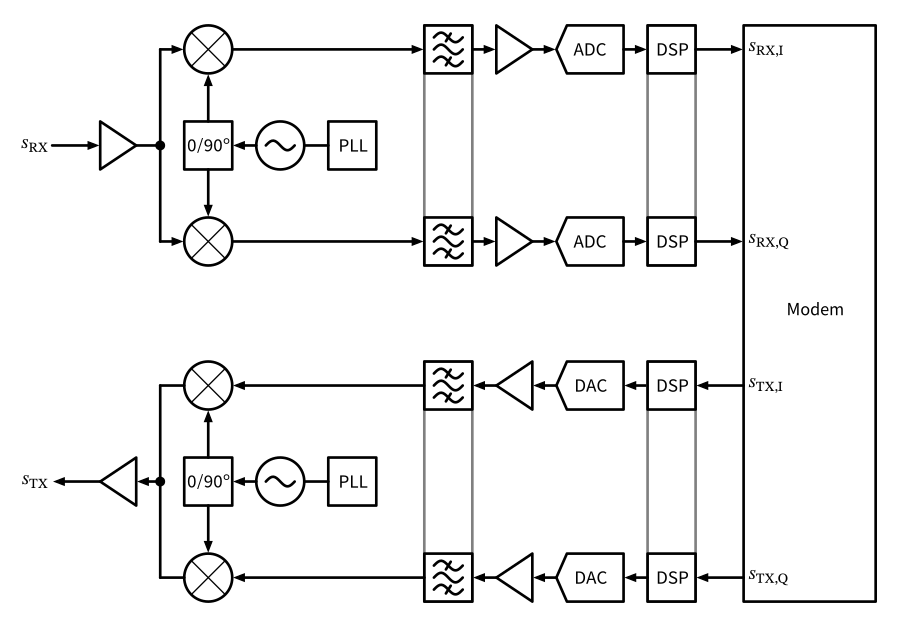
Figure 28: Block diagram of a low-IF transceiver (TRX) showing the main functional blocks of RX and TX.

Block diagram of a low-IF transceiver (TRX) showing the main functional blocks of RX and TX. Note the usage of complex analog and digital baseband filters. Otherwise, the structure is similar to a zero-IF TRX as shown in Figure 19.

3.6.3 Direct-Modulated Oscillator and Direct-Detection Receiver (aka “Super Simple” Architecture)

The low-IF architecture is the de facto standard for Bluetooth receivers. Its advantage compared to direct-conversion vanishes for larger channel bandwidths, which is why it is not used for cellular or Wi-Fi (GSM receivers might be an exception).

One noteworthy disadvantage of low-IF architectures is the required \(\ge 2\times\) BW of the analog baseband filters and the ADCs/DACs compared to direct-conversion. This might cause increased power consumption in these blocks. Additionally, the low-IF architecture still requires careful design to mitigate issues like I/Q imbalance and LO leakage, although these issues are generally less severe than in direct-conversion architectures.

For some applications with very low cost and low performance requirements, a super simple architecture can be used (for applications like a garage door opener). In this architecture, the RX and TX paths are stripped down to the bare minimum. A simple direct-detection receiver just uses an (optional) bandpass filter and a power detector, while a simple direct-modulated oscillator transmitter uses an oscillator and (optional) power amplifier. These simplified architectures are shown in Figure 29.

Direct-Modulated Oscillator and Direct-Detection Receiver (aka “Super Simple” Architecture)

Figure 29: Block diagram of a direct-modulated oscillator and direct-detection receiver (aka ‘Super Simple’) TX and RX with optional components.

3.7 I/Q Imbalance

Despite the reduced architecture, digital amplitude-shift-keying (ASK) or on-off-keying (OOK) can be used. If the receiver is able to discriminate between frequencies (e.g., by using two RF filters with a power detector each), also frequency-shift-keying (FSK) can be used.

I/Q Imbalance

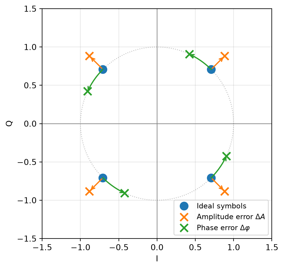
Figure 30: QPSK constellation illustrating the two error contributions.

In direct-conversion and low-IF architectures, the I and Q paths are used to process the in-phase and quadrature components of the signal. Ideally, these paths should have identical gain and a 90° phase difference. However, in practice, there are always some mismatches between the I and Q paths, leading to I/Q imbalance. This imbalance can cause constellation distortion, leading to increased error vector magnitude (EVM) and degraded system performance.

QPSK constellation illustrating the two error contributions. Applied to all four symbols, an amplitude error \(\Delta A\) (radial displacement, orange crosses) and a phase error \(\Delta \varphi\) (rotation on the circle, green crosses) are shown separately relative to the ideal symbols (blue circles).

I/Q Imbalance

• Image rejection ratio (IRR): The IRR is a measure of how well the receiver can reject the image frequency caused by I/Q imbalance. It is defined as the ratio of the power of the desired signal to the power of the image (unwanted) signal, typically expressed in dB. A higher IRR indicates better performance, with values above 30 dB to 40 dB generally considered acceptable for most applications.

I/Q imbalance can be characterized by two parameters: amplitude mismatch (\(\Delta A\)) and phase mismatch (\(\Delta \varphi\)). Amplitude mismatch originates from the difference in gain between the I and Q paths, while phase mismatch refers to the deviation from the ideal 90° phase difference. The impact of I/Q imbalance on system performance depends on the modulation scheme used, with higher-order modulations being more sensitive to these impairments. Figure 30 illustrates both effects on a QPSK constellation: an amplitude mismatch displaces each symbol radially, while a phase mismatch rotates each symbol along the constellation circle.

There are two ways to quantify I/Q imbalance:

The IRR can be calculated from the relative amplitude mismatch \(\epsilon = \Delta A/A\) and the phase mismatch \(\Delta \varphi\) (in radians) as (Razavi 2011)

I/Q Imbalance

\[ \begin{split} \text{IRR} &= \frac{1 + (1 + \epsilon)^2 + 2 (1 + \epsilon) \cos(\Delta \varphi)}{1 + (1 + \epsilon)^2 - 2 (1 + \epsilon) \cos(\Delta \varphi)}\\ &\approx \frac{4}{\epsilon^2 + (\Delta \varphi)^2}, \end{split} \tag{29}\]

where the approximation on the right holds for small amplitude and phase errors. The IRR in dB is given by

I/Q Imbalance

\[ \text{IRR}|_\mathrm{dB} = 10 \cdot \log_{10}(\text{IRR}). \]

For example, an amplitude mismatch of 1% (\(\epsilon = 0.01\)) together with a phase mismatch of 1° (\(\Delta \varphi \approx 0.0175\)) yields an IRR of about 40 dB.

I/Q Imbalance

• Error vector magnitude (EVM): The EVM is a measure of the difference between the ideal transmitted signal and the received signal, expressed as a percentage of the signal’s magnitude. It quantifies the overall distortion in the received signal, including the effects of I/Q imbalance. Lower EVM values indicate better performance, with typical requirements ranging from 1% to 10% depending on the modulation scheme and application.

The EVM (in rms) is defined as

I/Q Imbalance

\[ \text{EVM} = \frac{\sqrt{\frac{1}{N} \sum_{i=1}^{N} |s_{\mathrm{ideal},i} - s_{\mathrm{meas},i}|^2}}{\sqrt{\frac{1}{N} \sum_{i=1}^{N} |s_{\mathrm{ideal},i}|^2}} \tag{30}\]

\[ \text{EVM}|_\mathrm{dB} = 20 \cdot \log_{10}(\text{EVM}). \]

where \(s_{\mathrm{ideal},i}\) are the ideal transmitted symbols, \(s_{\mathrm{meas},i}\) are the measured received symbols, and \(N\) is the number of symbols. EVM is expressed either in percent or in dB using

Note that the EVM (in dB) is always a negative number, with lower values indicating better performance. For example, an EVM of 1% (a very good number) corresponds to –40 dB, while an EVM of 10% corresponds to –20 dB. The SNR of the RF signal can be related to the EVM as

I/Q Imbalance

\[ \text{SNR}|_\mathrm{dB} \approx -20 \cdot \log_{10}(\text{EVM}) = -\text{EVM}|_\mathrm{dB}. \]

In order to make the I/Q mismatch sufficiently small, the following techniques can be used:

• Careful layout and matching of the components in the I and Q paths to minimize gain and phase mismatches. This usually involves good layout techniques. Further, the LO I/Q generation should be done with high accuracy.
• Calibration techniques can be used to measure and compensate for I/Q imbalance. This can be done either in the analog domain (e.g., using variable gain amplifiers and phase shifters) or in the digital domain (e.g., using digital signal processing algorithms). Digital compensation is usually preferred, as it is more flexible and can adapt to changing conditions. A CORDIC can be readily used for this purpose.

I/Q Imbalance

• Careful layout and matching of the I and Q paths, accurate LO I/Q generation
• Calibration in the analog domain (VGAs, phase shifters) or, preferably, the digital domain (e.g., CORDIC)

References

Fulde, Michael, Alexander Belitzer, Zdravko Boos, et al. 2017. “13.2 a Digital Multimode Polar Transmitter Supporting 40MHz LTE Carrier Aggregation in 28nm CMOS.” 2017 IEEE International Solid-State Circuits Conference (ISSCC), February, 218–19. https://doi.org/10.1109/isscc.2017.7870339.

Gebhard, Andreas, Oliver Lang, Michael Lunglmayr, et al. 2019. “A Robust Nonlinear RLS Type Adaptive Filter for Second-Order-Intermodulation Distortion Cancellation in FDD LTE and 5G Direct Conversion Transceivers.” IEEE Transactions on Microwave Theory and Techniques 67 (5): 1946–61. https://doi.org/10.1109/tmtt.2019.2896513.

Martin, Kenneth W. 2004. “Complex Signal Processing Is Not Complex.” IEEE Transactions on Circuits and Systems—I: Regular Papers 51 (9): 1823–36. https://doi.org/10.1109/tcsi.2004.834522.

Molisch, Andreas F. 2022. Wireless Communications: From Fundamentals to Beyond 5G. 3rd edition. Wiley-IEEE Press.

Razavi, Behzad. 2011. RF Microelectronics. 2nd edition. Pearson.

Sadjina, Silvester, Christian Motz, Thomas Paireder, Mario Huemer, and Harald Pretl. 2020. “A Survey of Self-Interference in LTE-Advanced and 5G New Radio Wireless Transceivers.” IEEE Transactions on Microwave Theory and Techniques 68 (3): 1118–31. https://doi.org/10.1109/TMTT.2019.2951166.

Schaumann, Rolf, Haiqiao Xiao, and Mac E. Van Valkenburg. 2009. Design of Analog Filters. Second. Oxford University Press.

Sklar, Bernard, and Fredric J. Harris. 2020. Digital Communications: Fundamentals and Applications. 3rd edition. Pearson.

Zverev, Anatol I. 1967. Handbook of Filter Synthesis. John Wiley & Sons.

A final note on EVM: EVM is not only affected by I/Q imbalance, but also by other impairments like phase noise, nonlinearities, and noise in general. Therefore, EVM is a more comprehensive measure of the overall performance of a communication system, and often used to quantify the overall system performance in terms of SNR.

References