
VLSI Design
1 Introduction
This is the material for an introductory-level course on digital very-large-scale integration (VLSI) design, held at JKU under course number 336.051 (“KV: VLSI Design”).
The course teaches the design of digital application-specific integrated circuits (ASICs) with a modern, fully open-source RTL-to-GDSII flow, from the register-transfer level (RTL) to the layout. We model hardware in SystemVerilog, verify it with cocotb (Python), inspect waveforms in GTKWave/Surfer, and harden a design and assemble it into a complete, tapeout-ready chip, including the padframe, with LibreLane on the IHP SG13CMOS5L 130 nm open process design kit (PDK). In the course project, you take your own RISC-V system-on-chip (SoC) all the way to a tapeout-ready chip.
Important
All course material (the source of this document, the SystemVerilog code, the cocotb testbenches, the LibreLane configurations, and the Python sources for all figures) is made publicly available on GitHub (follow this link) and shared under the Apache-2.0 license.
Please feel free to submit pull requests on GitHub to fix errors and omissions!
Important
Please use the IIC-OSIC-TOOLS image with tag 2026.10 or later. It contains all tools and the PDK used in this course. Inside the container, echo $IIC_OSIC_TOOLS_VERSION prints the tag. An existing container keeps its image when it is started again, so to update, remove the container (the .sh start scripts offer this, the .bat scripts print the command), pull the new image with docker pull hpretl/iic-osic-tools:latest, and run the start script again. Your designs in /foss/designs are kept (Section 1.13.1).
1.1 Preamble on the Use of AI
Artificial intelligence offers impressive possibilities today: it can explain how things are connected, provide examples, help with debugging, or point out different ways to solve a problem. Precisely for this reason, however, there is a risk of relying too heavily on such tools while learning, and thereby not practicing enough of exactly those skills that this course is meant to build.
In the written exam, you will have to solve problems without any technical aids. There, the only thing that counts is which concepts, methods, and skills you have mastered yourself. Likewise, in the oral presentation of your project, you have to be able to explain what you did and why you did it.
If you want to complete a long-distance run in a few months, you have to build up your own endurance. You could, of course, cover your weekly training route faster on an e-scooter, but that does not train your ability to run the distance yourself. The same holds for your studies: if AI regularly does the actual thinking for you, you will not sufficiently build up the skills you need.
So feel free to use AI as a learning partner, but not as a substitute for your own thinking. Always try to understand and solve a problem on your own first. Afterwards, use AI, for example, to check your solution, to learn about an alternative approach, or to have a difficult topic explained to you. The goal of this course is not to arrive at a correct answer as quickly as possible, but to develop the competence to get there on your own.
In the end, you are here to learn something, so do not cheat yourself! This matters beyond the course, too: as AI agents take over more and more routine design work (see Section 1.11), engineers who know how to prompt these tools and, above all, how to critically review their results will always be needed. And you can only review what you understand yourself.
1.2 Learning Objectives
After completing this course, you will be able to:
- work with the IIC-OSIC-TOOLS container and manage your designs with Git and GitHub
- read and write synthesizable SystemVerilog RTL for synchronous digital designs, and translate idiomatic VHDL into idiomatic SystemVerilog
- apply modeling guidelines that make RTL ready for an ASIC (a simulation that matches the netlist, resets, no FPGA habits, registered macro boundaries, the right architecture)
- verify RTL with self-checking cocotb testbenches and reason about coverage and corner cases
- explain how logic synthesis maps RTL onto a standard-cell library, and prove the resulting netlist equivalent to the RTL with logic equivalence checking (LEC)
- analyze timing using the concepts of setup/hold, propagation delay, clock skew, and static timing analysis (STA), and write the timing constraints that STA checks against
- reduce the dynamic power of a design with clock gating
- handle multiple clock domains and resets safely with synchronizers and reason about metastability
- explain design for test (DFT), the stuck-at fault model, scan chains, and test coverage
- understand and explain the RTL-to-GDSII flow (synthesis, floorplanning, placement, clock tree synthesis, routing, signoff) and drive it with LibreLane
- integrate a digital macro into a padframe and assemble a complete, tapeout-ready ASIC with open-source tools
- design, verify, harden, and document a RISC-V SoC with your own extension as a capstone project
- optionally, use large language model (LLM) agents efficiently, and critically, in a chip design workflow
1.3 Prerequisites
The course is an elective for students of the Bachelor’s program in Computer Science and of the Master’s program in Electronics and Information Technology (ELIT). To follow it, you should bring:
- a basic understanding of CMOS transistors
- a good understanding of digital logic (gates, flip-flops, etc.)
- basic experience with a hardware description language (e.g., VHDL)
- your own laptop with at least 20 GB of free disk space for VS Code, Git, and the IIC-OSIC-TOOLS (see Section 1.13)
The following JKU courses, whose material is also openly available, complement this course well regarding silicon theory, transistor-level design, design methodologies, and layout rules, but are not required:
- KV Analog Circuit Design: https://github.com/iic-jku/analog-circuit-design
- KV Design of Complex Integrated Circuits: https://github.com/iic-jku/design-complex-ic
The following JKU courses complement this course well regarding digital design with VHDL, computer architecture and RISC-V, but are not required:
- VL+UE Computer Architecture: https://studienhandbuch.jku.at/199475
- PR Hardware Design Lab: https://studienhandbuch.jku.at/199477
1.4 Course Content
After this introduction, the course covers the following topics:
- hardware description with SystemVerilog, and modeling guidelines for synthesizable RTL (Section 2, Section 3)
- functional verification with cocotb (Section 4)
- logic synthesis, the standard-cell library, and logic equivalence checking (Section 5)
- sequential elements, static timing analysis, and timing constraints (Section 6)
- synthesis optimizations and low-power design (Section 7)
- clock domain crossing and resets, and design for test (Section 8, Section 9)
- the RTL-to-GDSII flow with LibreLane, chip assembly, and padframe (Section 10)
- the project: a tapeout-ready RISC-V SoC (Section 11)
The appendix lists possible questions for the written exam (Section 12).
NoteFurther Reading
These notes are self-contained but kept concise. For depth we recommend:
- (Harris and Harris 2021) for digital design and RISC-V computer architecture.
- (Weste and Harris 2010) for CMOS VLSI design from circuits to systems.
- (Cummings 2008) for clock-domain-crossing techniques in SystemVerilog.
1.5 Grading
The grade consists of two equally weighted parts:
- Part 1, Theory (50 %): The theoretical lectures are mixed with small examples. This part is assessed by a written exam before Christmas, on December 17, 2026. The exam is closed book, allows no technical aids, and is based on the questions in Section 12, partly with other numbers, circuits, or code.
- Part 2, Project (50 %): You implement a complete, tapeout-ready RISC-V SoC with your own extension (analog or digital) and present your work in an oral presentation (Section 11).
Tip
The best project might actually be taped out! Moreover, the project can be extended into a seminar work (+3 ECTS) or a thesis.
1.6 Why ASICs?
Application-specific integrated circuits are designed when standard, off-the-shelf components cannot meet the requirements. Typical motivations are:
- Specification: performance, power, or size targets unreachable with standard parts.
- Integration: combining digital logic, analog circuits, and on-chip memory into a single mixed-signal chip.
- Economics: at high volume the per-unit cost drops dramatically, and integrating more functionality into one chip reduces system cost.
Historically, the cost per transistor has fallen by orders of magnitude as integration density doubled roughly every 18 to 24 months (Moore’s law). What was once only affordable to large companies is, with open-source PDKs and tools, now accessible to students and researchers.
1.7 A Taxonomy of ASICs
ASIC implementation styles trade off non-recurring engineering (NRE) cost, unit cost, performance, and design effort. Table 1 compares them, from programmable logic devices (PLDs) and field-programmable gate arrays (FPGAs) to full-custom ICs. The more masks and design effort a style needs, the higher its NRE cost, and the lower its unit cost at high volume.
| Style | Masks | Effort | NRE / unit cost | Typical use |
|---|---|---|---|---|
| PLD / FPGA | none | low | lowest / highest | prototypes, low volume |
| Gate array / sea-of-gates | only wiring layers | medium | low / medium | medium volume |
| Standard-cell IC (CBIC) | all layers | medium to high | high / low | the workhorse of digital design |
| Full-custom IC | all layers, hand-crafted | very high | highest / lowest | highest performance |
This course focuses on the standard-cell style: we describe behavior in SystemVerilog and let the synthesis tool map it onto a library of pre-characterized standard cells from the SG13CMOS5L PDK (IHP GmbH 2026).
1.8 The Digital Design Flow
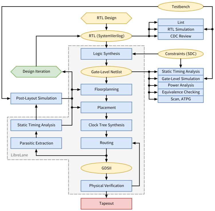
The core of this course is the digital design flow that turns a hardware description into a manufacturable layout. Since this layout is traditionally handed over to the foundry in the GDSII file format, it is called the RTL-to-GDSII (or simply RTL-to-GDS) flow. Figure 1 shows its main steps.
The flow starts with the RTL design, described in a hardware description language (HDL) such as SystemVerilog. Long before any layout exists, the RTL is checked: lint finds suspicious code without running it, RTL simulation runs it against a testbench, and designs with several clocks need a review of their clock domain crossings (CDC) (Section 8).
Logic synthesis translates the RTL into a gate-level netlist of standard cells of the target technology, guided by constraints such as the clock frequency, written in SDC (Synopsys Design Constraints). The netlist is checked as well: static timing analysis (STA) checks the timing of every path with an ideal clock, gate-level simulation (pre-layout simulation) repeats the tests with the same testbench, power analysis estimates the power consumption, logic equivalence checking proves that the netlist implements the RTL, and design for test inserts scan chains and generates test patterns (automatic test pattern generation, ATPG), so that every fabricated chip can be tested (Section 9). Every bug found here leads back to the RTL.
The physical implementation then turns the netlist into a layout. Floorplanning defines the size of the die and the core, the placement of I/Os and macros, and the power grid. Placement positions the standard cells, clock tree synthesis (CTS) builds a balanced clock distribution network, and routing connects all cells with metal wires.
Only after routing are the resistances and capacitances of the wires known. Parasitic extraction annotates them to the netlist, on which STA and post-layout simulation check whether the design still meets its timing and functional specification. Violations are fixed by revisiting floorplanning and placement or, if this is not enough, by changing the RTL itself (design iteration), e.g., by pipelining a critical path. Finally, the layout is written in the GDSII format, and physical verification checks it against the design rules of the foundry (design rule check, DRC) and against the netlist (layout versus schematic, LVS). A failed check leads back to routing. Only a design that passes all checks goes to tapeout, i.e., is sent to the foundry for fabrication.
LibreLane (Section 10) runs the steps in the dashed region of Figure 1. In this course, the checks beside it run separately, although LibreLane also runs lint and STA on its own. For a complete chip, the hardened digital macro is finally integrated into a padframe and assembled into the chip top level (Section 10). Table 2 lists the open-source tools used in this course for each step and where the step is covered.
| Flow step | Open-source tool | Covered in |
|---|---|---|
| HDL | SystemVerilog | Section 2, Section 3 |
| Lint | Verilator | Section 2, Section 3 |
| RTL, pre- and post-layout simulation | cocotb or a SystemVerilog testbench with Icarus Verilog, or Verilator for RTL, waveforms in GTKWave or Surfer | Section 4, Section 10 |
| CDC review | by hand, no tool in this course | Section 8 |
| Logic synthesis | Yosys | Section 5, Section 7 |
| Logic equivalence checking | EQY, Yosys equiv_* commands |
Section 5, Section 9, Section 10 |
| Scan insertion and test generation | OpenROAD, Fault | Section 9 |
| Floorplanning, placement, CTS, routing | OpenROAD | Section 10 |
| Parasitic extraction | OpenRCX | Section 10 |
| Static timing analysis | OpenSTA | Section 6, Section 10 |
| Power analysis | OpenSTA | Section 7 |
| Physical verification | Magic and KLayout (DRC), Netgen and KLayout (LVS) | Section 10 |
| Chip assembly and padframe | LibreLane with the AMS chip template | Section 10, Section 11 |
1.9 The IIC-OSIC-TOOLS Container
The legacy version of this course relied on commercial tools (Vivado, ModelSim, Synopsys Design Compiler, Cadence Innovus, TetraMAX, PrimeTime). This edition is built entirely on open-source tools, all pre-installed in the IIC-OSIC-TOOLS container (Institute for Integrated Circuits and Quantum Computing, JKU 2026). This all-in-one Docker/Podman image for analog and digital IC design is curated at JKU and runs natively on x86_64 and arm64 machines (e.g., Apple Silicon). Since everyone uses the identical container, results are reproducible, and “works on my machine” problems disappear.
As Table 3 shows, the container covers much more than this course needs: full-custom (analog) design with schematic entry, analog simulation, layout, and electromagnetic (EM) simulation, semi-custom (digital) design with simulation, synthesis, and complete RTL-to-GDSII flows, as well as several open-source PDKs. In this course, we mainly use the digital tools (Table 2) with the IHP SG13CMOS5L PDK, and the analog tools appear in the AMS chip template (Section 1.10).
| Category | Tools and PDKs |
|---|---|
| Schematic entry | Xschem, Qucs-S |
| Analog simulation | ngspice, Xyce, VACASK, CACE |
| Layout editing | Magic, KLayout, GDSFactory |
| Digital simulation and waveforms | Icarus Verilog, Verilator, cocotb, GTKWave, Surfer |
| Logic synthesis | Yosys (with the slang and GHDL front ends), ABC |
| RTL-to-GDSII flows | LibreLane, OpenROAD Flow Scripts, SiliconCompiler, QFlow |
| Place and route, STA, extraction | OpenROAD, OpenSTA, OpenRCX |
| DRC, LVS, and parasitic extraction | Magic, KLayout, Netgen, KLayout-PEX |
| EM simulation | Palace, openEMS |
| PDKs | sky130A, gf180mcuD, ihp-sg13g2, ihp-sg13cmos5l |
1.9.1 Open-Source and Commercial Tools
Industry builds most chips with commercial tools, and you will meet their names in job descriptions. Table 4 lists examples of them for each step of the flow and the main gap of the open-source tool. Many of its terms come up only in later chapters (Table 2 says where), so take it as a reference to come back to. This course does not use OpenCDC (OpenCDC developers 2026), Difetto (Gaber 2026), or read_upf, which reads the Unified Power Format (UPF). We ran no commercial tools: the table rests on public documentation, on runs of the open-source tools, and on the two comparisons below.
The gaps are of two kinds. The first is missing features. Some of them matter more in an advanced node or a large chip than in the small blocks of this course at 130 nm, e.g., crosstalk, where a switching neighbor changes the delay of a wire, dynamic IR drop, the short dips of the supply voltage when many cells switch at once, and electromigration, the wear of a wire at a high current density.
The second is the quality of the results. For a finite-state machine at 50 MHz in the IHP 130 nm open PDK, with the same constraints and the same switching activity, an open-source flow with Yosys and OpenROAD needed 53 % more area and 118 % more power than a commercial flow with Cadence Genus and Innovus (Freitas et al. 2025). An earlier comparison of RISC-V designs reports 1.24 times the area of a commercial tool after synthesis with Yosys at 130 nm and 1.49 times at 40 nm. Yosys ran faster than the commercial tool there, while the place-and-route steps of OpenROAD took 2.13 times as long (Sánchez Lopera et al. 2022).
All of this is a snapshot of tools that change quickly. Both comparisons used older tool versions, and within weeks after image 2026.10 was built, OpenSTA gained an experimental crosstalk delay analysis, which needs library models that SG13CMOS5L does not have, and OpenROAD a reordering of the scan chains. The script scripts/check_intro.sh tests what it can of the table in the image, and the sv-tests results show the language coverage of each tool.
2026.10
| Flow step | Open-source tool | Commercial tools (examples) | Main gap of the open-source tool |
|---|---|---|---|
| Lint | Verilator | Synopsys VC SpyGlass, Siemens Questa Lint | No testability rules, configurable naming rules only in Verible |
| Simulation | Icarus Verilog, Verilator | Cadence Xcelium, Synopsys VCS, Siemens Questa One Sim | Verilator: two-state, no SDF. Icarus Verilog: no SDF timing checks. Neither covers all of SystemVerilog |
| Clock domain crossings (CDC) | OpenCDC | Siemens Questa CDC, Synopsys VC SpyGlass CDC | Under development: false errors on correct designs, missed crossings (Section 8.7) |
| Logic synthesis | Yosys, ABC | Synopsys Design Compiler, Cadence Genus | Larger area, higher power, retiming only through ABC |
| Logic equivalence checking | EQY, Yosys equiv_* |
Cadence Conformal, Synopsys Formality | Language coverage of the Yosys front ends, the EQY step of LibreLane prepares cell models only for sky130 |
| Scan and test generation | OpenROAD, Fault, Difetto | Synopsys TestMAX, Siemens Tessent | Stuck-at faults only. Fault: mostly on whole nets. Difetto: early stage, not in the image (Section 9.7) |
| Place and route | OpenROAD | Cadence Innovus, Synopsys Fusion Compiler | Larger area, higher power, longer run times |
| Parasitic extraction | OpenRCX | Cadence Quantus, Synopsys StarRC | Rule-based, accuracy depends on the calibrated rules of the PDK |
| Static timing analysis | OpenSTA | Synopsys PrimeTime, Cadence Tempus | No crosstalk delay analysis |
| Power analysis | OpenSTA | Synopsys PrimePower, Cadence Voltus, Cadence Joules | Average power only, no peak power, no estimate at RTL |
| IR drop and electromigration | OpenROAD (PDNSim) | Cadence Voltus | Static IR drop of the power grid only, no electromigration limits, no signal wires |
| DRC and LVS | Magic, KLayout, Netgen | Siemens Calibre, Cadence Pegasus, Synopsys IC Validator | A commercial PDK usually ships its rule decks only for commercial tools |
| Power intent (UPF) | OpenROAD read_upf |
Cadence Conformal Low Power, Synopsys VC LP | Subset of UPF, no open-source UPF checker known to us |
For this course, the gaps are a fair price. Every student gets the same tools without a license or a non-disclosure agreement, you can read what each tool does, and the flow takes a design all the way to tapeout (Section 1.12).
1.10 The AMS Chip Template
Hardening a single digital block is only part of the way to a chip. A tapeout-ready chip additionally needs a padframe and a seal ring, the placement and wiring of all macros on the top level, logo and metal-fill insertion, full-chip verification, and finally a bonding diagram for packaging. To get there without fighting the tools, this course builds on the ihp-sg13cmos5l-ams-chip-template (Dorrer and Pretl 2026), an open-source GitHub template repository for analog mixed-signal (AMS) chips developed at JKU:
- It is released under the permissive Solderpad Hardware License v2.1.
- Create your own repository with GitHub’s Use this template button (or simply
git cloneit), enter the IIC-OSIC-TOOLS container, and runmake all. The result is a tapeout-ready AMS chip. - A step-by-step tutorial, written in Quarto, walks through all IC design steps on IHP’s 130 nm process, with simple exercises to learn by doing. You start your project with this tutorial (Section 11).
- Regression tests via GitHub Actions ensure that the flow keeps working with every new release of the tools.
The template is also available for the ihp-sg13g2, sky130A, and gf180mcuD open PDKs, and several chips have already been taped out with it, including TinyWhisper (Section 1.12).
1.10.1 Flow Overview
The Makefile-driven flow of the template covers:
- simulation, linting, and hardening of the RTL
- layout checks and reports of the hardened digital macro
- simulation of all analog testbenches, including process, voltage, and temperature (PVT) corners and Monte Carlo (MC) analysis
- layout checks of the analog and digital blocks (DRC, LVS, and parasitic extraction, PEX)
- digital-on-top assembly of the chip top level and its layout check (DRC), including
- seal ring and padframe generation
- macro placement and wiring, also with non-default rules (NDRs)
- logo and fill insertion
- full top-level LVS and simulation without black-boxing
- generation of the bonding diagram
1.10.2 Folder Structure and Makefiles
The folder structure of the template was discussed with the FOSSi community. Every macro in macros/ (e.g., the digital counter and the analog inverter examples) follows the same scheme as the chip top level, with its own Makefile and folders such as rtl/, testbenches/, schematic/, layout/, netlist/, verification/, and final/. Since a macro can itself contain macros, the structure is recursive. This makes it easy to share macros between projects and to reproduce the results of others.
At the top level, make all runs four steps:
make build-allbuilds the bondpad, the logos, all enabled macros, and finally the chip top level (LibreLane assembly, reports, GDS, netlists, logo and fill insertion, and renders)make magic-drc(ormake klayout-drc) checks the final layout of the chipmake sim-allsimulates the chip (RTL and gate-level simulation with cocotb, gate-level simulation with Xschem)make bondplangenerates the bonding diagram for packaging
Targets that build an intellectual property (IP) block or a macro recursively call the Makefile of that block.
1.11 Agentic AI Chip Design
Large language model (LLM) agents are increasingly able to operate a complete chip design environment: they do not only answer questions, but also edit design files, run tools, interpret the results, and iterate. Figure 2 shows such an agentic workflow.

make open (shown here for the SG13CMOS5L version of the AMS chip template).
The designer interacts with the LLM agent through prompts and reviews. The agent can be any coding agent that reads files and runs commands in a terminal. It edits the RTL, schematics, and layout of a chip project based on the AMS chip template (Section 1.10) and runs its make targets, which call the tools of the IIC-OSIC-TOOLS. The results of simulation, DRC, LVS, and PEX flow back to the agent and to the designer.
The agent uses the tools in the same way as a designer in a terminal, which allows it to iterate without help. The tools of the flow run without a graphical user interface (GUI): Xschem exports netlists in batch mode, and ngspice, KLayout, Magic, Netgen, and LibreLane run from a script or a configuration file. The template has one make target for each flow step, so the agent runs, for example, make sim-gl-cocotb, make klayout-drc, make magic-lvs, make klayout-pex, or make librelane, reads the resulting logs and reports, fixes the design, and runs the target again. make help lists all targets with their parameters, so an agent can find its way around a new project on its own. The designer can reproduce every reported result with a single command.
The designer stays in the loop. Where it is faster, they edit the project by hand, and they check the tool results themselves (the dashed arrows labeled manual edits and manual review in Figure 2). Both paths go through make open, which starts a small Python GUI from the IIC-OSIC-TOOLS with one button per design file. A click opens the file in its tool, for example a schematic in Xschem or a layout in KLayout. This target needs a display, so run it on the VNC desktop of the container or over X11.
All changes are tracked in version control (e.g., Git and GitHub). The agent creates branches, commits and pushes changes, sets up continuous integration (CI) workflows, and opens pull requests, so each of its changes is a diff. The designer reviews these diffs and decides what is pushed, merged, or deleted.
A knowledge base (an index plus notes) lets the agent learn across sessions. The agent searches the index first and reads only the notes relevant to the task, which keeps its context small. At the end of a session, it distills what it learned, that is, decisions and their reasons instead of raw logs, back into the notes and updates the index, so that the next session can build on it, in any project and with any agent.
Such a workflow is only possible because every step of the flow is scripted, every tool runs in a reproducible container, and every result is machine-readable. Note the role of the designer: they remain responsible for the design and have to judge whether the results of the agent are correct, which brings us back to Section 1.1. Using LLM agents efficiently is an optional learning objective of this course.
1.12 Example: The TinyWhisper SoC
What is possible with open-source tools and the AMS chip template is demonstrated by TinyWhisper, an open-source, fully integrated, multi-mode short-wave transmitter for amateur radio, developed in a cooperation between JMU Würzburg and JKU Linz. TinyWhisper combines a RISC-V CPU with peripherals, custom digital signal generation, and an analog front-end on one chip, so it is a good preview of what you will build in the course project. The block diagram and all design files can be found in the repository, and the full documentation is available online.
1.12.1 Weak Signal Propagation Reporter
TinyWhisper targets the Weak Signal Propagation Reporter (WSPR) protocol, a popular digital mode in amateur (ham) radio for propagation studies in the 80 m to 10 m bands. A WSPR transmitter sends a short message (callsign, location, and transmit power) using 4-FSK modulation with a tone spacing of \(\Delta f = 1.46\,\mathrm{Hz}\) and a symbol duration of \(T = 0.683\,\mathrm{s}\). Receivers can decode signals down to a signal-to-noise ratio of \(-31\,\mathrm{dB}\) in a 2500 Hz bandwidth and report everything they receive to a central database via the Internet (WSPRnet map). On TinyWhisper, the modem part (coding, framing, and symbol mapping) is implemented in firmware written in C, which runs on the on-chip RISC-V CPU.
1.12.2 Chip Overview
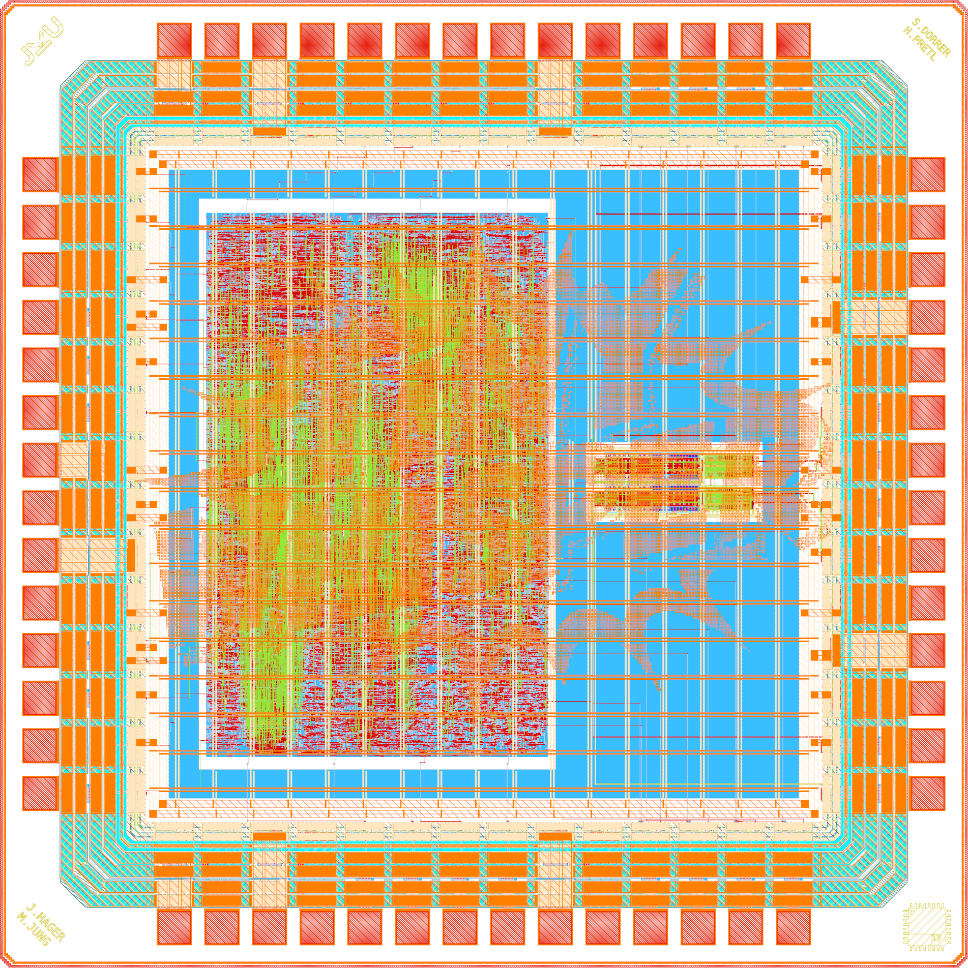
Table 5 summarizes the key parameters of the chip, and Figure 3 shows renders of its layout. The custom logo on the topmost metal layer (Figure 3 (b)) was generated with the tool ArtistIC of the PULP platform. TinyWhisper was taped out in the IHP open multi-project wafer (MPW) run in March 2026 and, at the time of writing (October 2026), is still in fabrication.

| Parameter | Value |
|---|---|
| Technology | IHP SG13CMOS (130 nm CMOS), open PDK |
| Die area | 2000 µm × 2000 µm (4 mm²) |
| Core area | 1270 µm × 1270 µm (1.61 mm²) |
| Clock frequency | 56 MHz |
| Core / I/O supply voltage | 1.5 V / 3.3 V |
| Pads | 56 |
| Package | QFN-48 (8 pads bonded directly to package ground) |
The digital core is built around an embedded RISC-V CPU implementing rv32e_zicsr, i.e., the 32-bit embedded base integer instruction set with 16 registers plus the extension for control and status registers. The CPU is a multi-cycle design without pipelining, running at 56 MHz, and accesses its SPI, I²C, UART, and GPIO peripherals as memory-mapped I/O. The IQ baseband signals are generated in hardware: a 30-bit iterative CORDIC computes sine and cosine with a frequency resolution of \(\Delta f = f_\mathrm{clk}/2^{30} \approx 0.05\,\mathrm{Hz}\), and a single-bit second-order delta-sigma modulator (oversampling ratio up to 256) converts its output into a bitstream for the analog front-end. Both are configurable via software. Furthermore, the digital core divides the clock down to the 25 % duty-cycle local oscillator (LO) signals of the mixers, which cover the 80 m, 40 m, 20 m, and 10 m bands.
The RISC-V CPU has already been proven in silicon: it was part of a multi-project student chip (with digital filters, mini games, and more) fabricated in the GlobalFoundries GF180MCU technology in the first wafer.space run (GitHub). On a breadboard, with the firmware supplied by an external microcontroller board and a discrete third-order multiple-feedback low-pass filter, the chip generates a clean baseband signal.
The analog front-end is an IQ modulator. Each of its two channels consists of a third-order multiple-feedback (MFB) Butterworth low-pass filter with a cutoff frequency of 400 kHz, built around a Barthélemy/Manfredini inverter-based operational transconductance amplifier (OTA), followed by a passive CMOS voltage-mode mixer with simple transmission-gate (TG) switches and a single-to-differential conversion circuit. Remarkably, the front-end consists only of inverter- and TG-based circuits. As an IQ transmitter, it supports not only WSPR but also other modes such as FT8, SSB, and CW.
Finally, even the bonding diagram for packaging is generated automatically: a Python script reads a configuration file with the pinout and placement, extracts the relevant layers (top metal and pads) from the layout, places the chip in the package, determines the pad centers, draws the bond wires, and renders the result as GDS. This is exactly what make bondplan of the AMS chip template does (Section 1.10.2).
“The aha moment of seeing your circuit come to life will stay long after the equations are forgotten.” (Peter Kinget)
1.13 Tools Installation
You can either install the IIC-OSIC-TOOLS locally on your own laptop or use a workspace on a JKU server via your browser.
1.13.1 Local Installation
Install Visual Studio Code from https://code.visualstudio.com.
Run the interactive installer. It sets up Git, Docker (or Podman), WSL2 on Windows or XQuartz on macOS, and clones the IIC-OSIC-TOOLS repository (by default to
~/iic-osic-tools). Every action asks for your confirmation first.On Windows, open PowerShell as Administrator and run:
irm https://osic.tools/install.ps1 | iexOn macOS and Linux, run:
curl -fsSL https://osic.tools/install.sh | bashReboot your computer. On Windows and macOS, start Docker Desktop once afterwards.
Start the container from within the
iic-osic-toolsfolder with.\start_vnc.bat(Windows) or./start_vnc.sh(macOS and Linux), and open http://localhost/?password=abc123 in your browser. The first start downloads the image (about 4 GB), so be patient. With Podman, the default port is 8080 instead of 80, and the start script always prints the correct URL. On macOS and Linux,./start_x.shalternatively shows the tools directly on your desktop via X11.Store your designs in
~/eda/designson your laptop (%USERPROFILE%\eda\designson Windows), which appears as/foss/designsinside the container. Only this folder persists when the container is removed or updated.
Tip
Piping a script from the Internet directly into a shell runs it without review. If you prefer to inspect the installer first, download it, read it, and run it locally, e.g., curl -fsSLO https://osic.tools/install.sh && less install.sh && bash install.sh.
1.13.2 Containerized On-Demand Workspace System (COWS)
If you cannot or do not want to install the tools locally, you can use the Containerized On-Demand Workspace System (COWS) instead, which provides a ready-to-use design environment in your browser:
- Open COWS at https://jku128011.riic.uni-linz.ac.at/.
- Log in with the credentials provided to you and change your password.
- Create a workspace: go to Workspaces, click Create workspace, enter a Workspace name, and select the KV VLSI Design 26/27 template.
- Start the workspace. Its Status should change to Running.
- Open the workspace by clicking its name.
Enjoy your workspace, and happy designing!
2 Hardware Description with SystemVerilog
Most of you already design digital circuits in VHDL. This chapter is a crash course that maps what you know from VHDL onto synthesizable SystemVerilog, the hardware description language (HDL) we use throughout this course. It is not an introduction to digital design: the synchronous, latch-free design style you learned with VHDL carries over unchanged, and only the syntax and a few semantic rules are new. Along the way, you write testbenches in SystemVerilog and in Python with cocotb, and you lint, simulate, and synthesize your designs in the IIC-OSIC-TOOLS container.
Note
All code of this chapter (RTL, VHDL references, testbenches, and the solutions of the exercises) is available in the folder content/sv_crashcourse/code of the course repository, with one folder per design. The SystemVerilog code follows the layout of a macro in the AMS chip template: the RTL in rtl/ and the testbenches in testbenches/verilog/ and testbenches/cocotb/. The VHDL versions are in vhdl/, the plain Verilog original of the priority encoder exercise is in verilog/, and the lint exercise keeps its file with deliberate mistakes in exercise/. Every file in rtl/ lints without warnings and synthesizes, and all testbenches pass with the tools of the IIC-OSIC-TOOLS image 2026.10: Verilator 5.052, Icarus Verilog 14.0, cocotb 2.1.0, GHDL 7.0.0-dev (for the VHDL files), and Yosys 0.70. With another image, the cell counts in the solutions can differ slightly. The script scripts/check_sv_crashcourse.sh reproduces every tool result of this chapter: run bash scripts/check_sv_crashcourse.sh in the container from the root of the repository.
For the exercises, clone the course repository into your designs folder once, if you have not done so yet:
cd /foss/designs
git clone https://github.com/iic-jku/vlsi-design.git
2.1 Learning Objectives
After this chapter, you will be able to:
- explain how a hardware description differs from software for a microcontroller
- describe a synchronous sequential circuit as a register plus next-state logic, and explain why the combinational logic has one clock period to compute
- name the main families of HDLs and judge their strengths and weaknesses
- translate VHDL designs written in the two-process style into idiomatic SystemVerilog
- read plain Verilog, e.g., netlists and older IP, and translate Verilog RTL into SystemVerilog
- write synthesizable combinational and sequential logic with
always_combandalways_ff, and avoid latches, races, and width errors - write self-checking testbenches in SystemVerilog and in Python with cocotb
- lint, simulate, and synthesize a design in the IIC-OSIC-TOOLS container by typing the commands yourself, and explain what the corresponding make targets of the AMS chip template do
2.2 Recap: Microcontroller Software versus Hardware Description
A C program for a microcontroller (MCU) and a SystemVerilog module may look alike: both have variables, operators, if, and for. Yet they describe fundamentally different things. The C program is a list of instructions that a fixed processor executes one after another. The program counter selects the next instruction, and the time a computation takes follows from the number of executed instructions. A hardware description, in contrast, describes the circuit itself. After synthesis, every line has become gates and flip-flops, and all of them work at the same time, all the time. Time is explicit: the registers update at the clock edge, and the combinational logic between them has one clock period to settle. Table 6 summarizes the differences.
| Aspect | Software for an MCU (e.g., C) | Hardware description (HDL) |
|---|---|---|
| What is described | a sequence of instructions for a fixed processor | the structure and behavior of the circuit itself |
| Execution | one instruction after another, controlled by the program counter | all statements and blocks operate concurrently, all the time |
| Time | implicit, follows from the number of instructions | explicit, every register updates at the clock edge |
| A variable is | a memory location or a CPU register | a wire (combinational logic) or a flip-flop, inferred from how it is assigned |
| A loop is | a repetition in time | a repetition in space: unrolled into parallel hardware, the bound must be a constant |
| A function call is | a jump to shared code | a separate copy of the hardware for every call |
| Compilation result | machine code in the flash memory | a netlist of gates and flip-flops, then a layout (GDSII) |
| Cost | memory and clock cycles | area, power, and maximum clock frequency |
| Debugging | debugger, printf, single steps on the target |
simulation and waveforms before the tapeout, little visibility in silicon |
| Fixing a bug | a firmware update | for an ASIC, a new mask set and fabrication run, which takes months |
The most important consequence is a change in thinking: think hardware first, then write the code. Before you write a module, sketch its block diagram with the registers and the combinational logic between them (Section 2.2.2). The code then only describes this diagram. Keep in mind that a simulator executes your HDL as an event-driven program on your computer. This is why HDLs also contain constructs such as delays, $display, or file access, which only make sense in simulation and cannot be synthesized (Section 2.5.12).
In the course project (Section 11), you need both ways of thinking. You build a RISC-V SoC: the CPU and the blocks around it are hardware that you describe as registers and combinational logic, and the CPU runs firmware that you write as for any microcontroller. Many SoCs today contain such a processor core, because the firmware keeps the digital part flexible: a new feature or a bug fix in the control flow needs a firmware update instead of a new mask set, while dedicated hardware handles the time-critical parts. RISC-V is a popular choice for this core, since its instruction set is open and can be used and extended without license fees. TinyWhisper (Section 1.12) is an example, with its modem in C firmware on the RISC-V CPU and its IQ modulator in dedicated hardware.
2.2.1 Computing in Time and in Space
The difference between software and hardware becomes obvious with a loop. The following C function counts the ones in a byte (population count):
uint8_t popcount(uint8_t x)
{
  uint8_t count = 0;
  for (int i = 0; i < 8; i++)
    count += (x >> i) & 1;
  return count;
}
In the loop body, (x >> i) & 1 shifts bit i of x into the least significant position and clears all other bits, so count grows by one exactly when bit i is set. The same function written in SystemVerilog looks almost identical, but the hardware behind it is not a loop at all:
popcount/rtl/popcount.sv
// SPDX-FileCopyrightText: 2026 Simon Dorrer
// SPDX-License-Identifier: Apache-2.0
// Description: Combinational population count (number of ones in x_i).

`default_nettype none

module popcount (
  input  logic [7:0] x_i,
  output logic [3:0] count_o
);

  // Add up the bits of x_i
  always_comb begin
    count_o = '0;
    for (int i = 0; i < 8; i++) begin
      count_o = count_o + 4'(x_i[i]);
    end
  end

endmodule

`default_nettype wire
In the loop body, x_i[i] selects bit i directly, without a shift and a mask, and the size cast 4'(...) (Section 2.5.3) extends this 1-bit value explicitly to the 4 bits of count_o, which SystemVerilog would otherwise do silently.
TipExercise: Loops in Software and in Hardware
- Roughly how many clock cycles does an MCU need for the C function? How long does the hardware need?
- What does the synthesis tool build from the
forloop inpopcount.sv? Is there a loop counteriin the hardware? - What changes in both cases when
xhas 64 bits instead of 8? - Optional, if you already have the container running: save the listing as
popcount.sv, synthesize it withyosys -p "read_verilog -sv popcount.sv; synth -top popcount; stat", and look at the cell statistics at the end of the log (Section 2.7.6 explains the command).
Before continuing, please finish the previous exercise. Once you are done, compare with the solution below.
TipSolution: Loops in Software and in Hardware
- Per iteration, the MCU executes a shift, an AND, an addition, the increment of
i, and a compare-and-branch, so about 40 instructions plus the function call. Depending on the core and the compiler, this takes several tens of clock cycles. The hardware needs no clock cycle at all: the module is purely combinational, and the result is valid after the propagation delay of the logic, usually well within one clock period of the surrounding registers. - The loop is unrolled at elaboration: the synthesis tool creates a chain of eight adders (and may restructure them into a tree, as long as the function stays the same). The loop variable
iexists only at compile time, so there is no counter in the hardware. This is why loop bounds in synthesizable code must be constants. - The MCU needs eight times as many iterations, so the time grows. The hardware needs eight times as many adders, and wider ones, so the area grows by more than a factor of eight. The result still needs no clock cycle, but the propagation delay grows as well, although an adder tree grows more slowly than a chain. This is the basic trade-off between computing in time and computing in space. Processors often add dedicated hardware for such functions, e.g., the
cpopinstruction of the RISC-V bit-manipulation extension Zbb. - Yosys 0.70 reports 26 generic logic cells (
$_XOR_,$_NAND_,$_ANDNOT_, and others) and no flip-flops, confirming that the module is purely combinational.
2.2.2 Synchronous Sequential Design
The popcount module is purely combinational: its output depends only on its current inputs. Most circuits also need memory, e.g., for the state of a finite state machine (FSM) or the value of a counter. Almost all of them are built as synchronous sequential circuits with the structure of Figure 4. A register of edge-triggered flip-flops stores the current state. The next-state logic, a purely combinational circuit, computes the next state from the current state and the inputs. At every rising clock edge, the register loads the next state from its D input, and the new state appears at its Q output. The outputs of the circuit are derived from the state (Moore FSM) or from the state and the inputs (Mealy FSM).
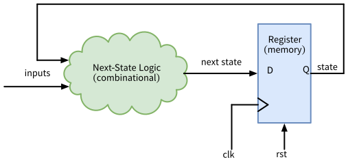
next_state_logic in VHDL, always_comb in SystemVerilog), and the register process describes the register (reg_proc in VHDL, always_ff in SystemVerilog).
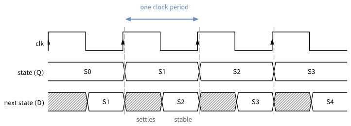
Edge-triggered flip-flops are the key to this structure. Their outputs change only at the rising clock edge and stay stable for the rest of the clock period. The next-state logic therefore sees stable inputs for one full clock period, and this is exactly the time it has to compute the next state. The result must have settled before the next rising edge (more precisely, a setup time before it), when the register loads it (Figure 5). The same holds for every path from a register through combinational logic to the next register, so the clock period only has to be longer than the slowest of these paths. Static timing analysis checks exactly this for every path in the design (Section 6). The rule assumes that the inputs also change only after a clock edge, i.e., that they come from registers driven by the same clock. An asynchronous input needs a synchronizer first (Section 8).
In your VHDL designs, you describe this structure with two processes, a register process reg_proc and a combinational process such as next_state_logic. As a minimal example, consider a toggle flip-flop, whose state inverts at every rising clock edge at which toggle_i is high:
-- Register process: only reset and clock in the sensitivity list
reg_proc: process(rst_i, clk_i) is
begin
  if rst_i = '1' then
    state <= '0';
  elsif rising_edge(clk_i) then
    state <= next_state;
  end if;
end process reg_proc;

-- Combinational process: all signals it reads in the sensitivity list
next_state_logic: process(state, toggle_i) is
begin
  -- default assignment
  next_state <= state;

  -- calculate next_state from state and the inputs
  if toggle_i = '1' then
    next_state <= not state;
  end if;
end process next_state_logic;
Three rules make this style work:
- The register process has only the reset and the clock in its sensitivity list, because the register reacts to nothing else. Its body is always the same: the reset values and, at the rising clock edge, the copies of the
next_signals. No logic belongs here. - The sensitivity list of the combinational process contains all signals that are read in the process. The simulator executes the process only when a signal in this list changes, while the synthesis tool ignores the list (at best with a warning) and builds combinational logic anyway. A missing signal therefore makes the simulation differ from the synthesized hardware. VHDL-2008 avoids this problem with
process(all). - The combinational process starts with a default assignment, here
next_state <= state, followed by all decisions. Every signal is thus assigned on every path, and no latch can arise. Keeping the state is not a latch: the register is the memory, and the next-state logic only feeds the current state back to its D input.
Section 2.5.7 shows the same style and the same three rules in SystemVerilog.
2.3 The HDL Landscape
VHDL and Verilog appeared in the 1980s, and for decades they were practically the only choice. In the last fifteen years, a large number of alternatives has appeared, most of them open source. They fall into four families:
- Standardized HDLs. VHDL (IEEE 1076), Verilog (IEEE 1364), and SystemVerilog (IEEE 1800, which absorbed Verilog in 2009) are read directly by the commercial simulation, synthesis, and verification tools. Among the open-source tools, (System)Verilog has much broader support than VHDL (Table 9).
- Embedded domain-specific languages (eDSLs), also called hardware construction languages. The hardware is described with a library of a general-purpose language such as Scala, Python, or Haskell. Running the program generates the hardware as Verilog, so the classes, functions, loops, and type system of the host language are available to build parameterizable generators.
- New standalone HDLs with their own syntax and compiler, designed to avoid the pitfalls of Verilog. They also emit (System)Verilog.
- High-level synthesis (HLS) and compiler intermediate representations. An algorithm written in C/C++ or a dataflow language is scheduled into clock cycles by the tool, or a compiler uses an intermediate language as its hardware back end.
Figure 6 shows how the four families relate.
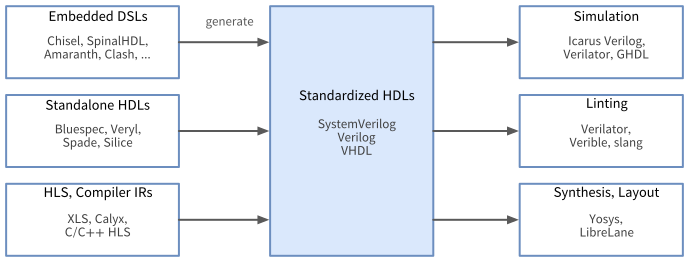
Table 7 gives an overview of the languages you are most likely to come across.
| Language | Family (host language) | Key idea | Origin | Output |
|---|---|---|---|---|
| VHDL | standard, IEEE 1076-2019 | strongly typed, deterministic signal semantics | US Department of Defense, IEEE standard since 1987 | read by commercial tools and GHDL |
| Verilog | standard, IEEE 1364-2005 | weakly typed, compact syntax | Gateway Design Automation, 1984 | read by all tools |
| SystemVerilog | standard, IEEE 1800-2023 | Verilog plus design and verification extensions | Accellera (2002), IEEE since 2005 | read by all tools |
| Chisel | eDSL (Scala) | generators, compiled through FIRRTL and CIRCT | UC Berkeley, 2012 | Verilog, SystemVerilog |
| SpinalHDL | eDSL (Scala) | generators | Charles Papon, 2015 | VHDL, Verilog |
| DFiant (DFHDL) | eDSL (Scala 3) | dataflow, timing-agnostic description | Technion, 2017 | Verilog, VHDL |
| Amaranth | eDSL (Python) | generators, successor of Migen (first called nMigen) | 2019, renamed in 2021 | Verilog via Yosys |
| Migen | eDSL (Python) | generators, still the base of the LiteX SoC builder | M-Labs, 2011 | Verilog |
| PyMTL3 | eDSL (Python) | modeling at functional, cycle, and RTL level | Cornell University, 2014 (as PyMTL) | Verilog |
| PyRTL | eDSL (Python) | minimal RTL for teaching and research | UC Santa Barbara, 2014 | Verilog |
| Magma | eDSL (Python) | strongly typed circuits | Stanford University, 2017 (inactive since 2024) | Verilog via CoreIR |
| Kratos | eDSL (Python) | generators with source-level debugging | Stanford University, 2019 (inactive since 2023) | SystemVerilog |
| HWT | eDSL (Python) | hardware construction library | Michal Orsák, 2015 | VHDL, Verilog, SystemC |
| Clash | eDSL (Haskell) | functional, signals as streams of values | University of Twente, 2009 | VHDL, Verilog, SystemVerilog |
| Hardcaml | eDSL (OCaml) | generators and expect tests | Andy Ray, Jane Street | Verilog, VHDL |
| ROHD | eDSL (Dart) | generator and verification framework | Intel, 2021 | SystemVerilog |
| RHDL | eDSL (Rust) | plain Rust code as hardware description | Samit Basu, 2023 | Verilog |
| Bluespec | standalone | rules as guarded atomic actions | Bluespec Inc., open source since 2020 | Verilog |
| Veryl | standalone | modernized SystemVerilog syntax with formatter, linter, and package manager | 2022 | SystemVerilog |
| Spade | standalone | Rust-like, pipelines as a language construct | Linköping University, 2020 | Verilog |
| Silice | standalone | algorithms, FSMs, and pipelines in a C-like syntax | Sylvain Lefebvre, 2019 | Verilog |
| XLS | HLS (DSLX or C++) | dataflow with automatic pipelining | Google, 2020 | Verilog, SystemVerilog |
| Calyx | compiler IR | intermediate language for accelerator compilers | Cornell University, 2021 | Verilog |
| C/C++ HLS | HLS (C, C++, SystemC) | untimed algorithm, scheduled into cycles by the tool | AMD Vitis HLS, Siemens Catapult, Bambu (open source) | Verilog, VHDL |
All non-standard languages have one thing in common: their output is Verilog or SystemVerilog (sometimes VHDL), which then goes through the same simulators and synthesis tools as hand-written RTL. (System)Verilog is the common exchange format of the whole industry. Table 8 compares the four families.
| Criterion | Standardized HDLs | Embedded DSLs | New standalone HDLs | HLS |
|---|---|---|---|---|
| Industry adoption | very high, the reference for all electronic design automation (EDA) tools, intellectual property (IP), and jobs | niche, some companies and many open-source cores (Rocket Chip and BOOM in Chisel, VexRiscv in SpinalHDL) | research and early adopters | established for data paths in commercial FPGA and ASIC flows |
| Tool support | all simulators, synthesis, lint, formal, and timing tools | host-language toolchain plus the generated Verilog | one compiler, few other tools | mostly commercial, open-source tools less mature |
| Abstraction and productivity | RTL, limited metaprogramming (parameters, generate) | high, the full host language builds generators | medium to high, modern syntax and type inference | highest, algorithmic description |
| Learning curve | moderate, Verilog has many pitfalls | host language plus hardware thinking | new syntax, small community and documentation | low for software developers, but good results need hardware knowledge and tool directives |
| Error checking | VHDL strongly typed, (System)Verilog weakly typed and dependent on lint | type systems of the host languages catch many errors | strong type systems, some prevent whole classes of bugs (e.g., races in Bluespec) | depends on the C model, timing is implicit |
| Debugging | source, waveform, and netlist correspond directly | generated Verilog with machine-made names | similar to eDSLs | the RTL is hard to relate to the source, latency depends on scheduling |
| Long-term risk | decades of stability | depends on small projects, several are dormant | early stage | lock-in to a vendor tool |
2.3.1 Why SystemVerilog in This Course
- Industry standard. SystemVerilog (IEEE 1800-2023 (IEEE 2024)) is the dominant language for ASIC design and verification. Every EDA tool, IP vendor, and foundry flow supports it.
- Open-source tool support. All tools of our flow read it: the simulators Verilator and Icarus Verilog (also under cocotb), Yosys and LibreLane, slang, and Verible. The AMS chip template (Section 1.10) is written in SystemVerilog.
- You have to read it anyway. Netlists, gate-level simulations, and the output of every alternative HDL are (System)Verilog. Debugging always ends there. Section 2.5.13 shows how plain Verilog maps onto SystemVerilog.
- cocotb for verification. The verification part of SystemVerilog (classes and constrained randomization) and the UVM library built on it form a large field of their own. With cocotb (Section 4), we write testbenches in Python and use SystemVerilog mainly for the synthesizable RTL.
- A good foundation. With solid RTL skills in SystemVerilog, you can learn an embedded DSL such as Chisel or Amaranth later with little extra effort, since it describes the same registers and logic.
2.3.2 VHDL versus SystemVerilog
Table 9 compares the two languages.
| Aspect | VHDL | SystemVerilog |
|---|---|---|
| Standard | IEEE 1076-2019 | IEEE 1800-2023, includes Verilog |
| Typing | strong, explicit conversions (numeric_std) |
weak, widths are extended or truncated silently, lint catches part of it |
| Verbosity | verbose (entity and architecture, type conversions) | compact |
| Case sensitivity | case-insensitive | case-sensitive (clk and Clk are different) |
| Simulation semantics | signals update after a delta cycle, the order of processes never matters | blocking and non-blocking assignments, races are possible if the coding rules are broken |
| Verification features | libraries (OSVVM, UVVM) | built in: classes, randomization, assertions (SVA), coverage, plus the UVM class library (IEEE 1800.2) |
| Typical use | FPGA, aerospace and defense, Europe, academia | ASIC design and verification worldwide |
| Open-source tools | GHDL (simulation), experimental synthesis via a Yosys plugin | Verilator, Icarus Verilog, Yosys, slang, Verible |
In short, VHDL protects you with strong typing, while SystemVerilog relies on coding discipline and on the linter. The rest of this chapter is about that discipline.
2.4 Cheat-Sheets, Guidelines, and Further Reading
Two cheat-sheets are provided with the AMS chip template:
- SystemVerilog Cheat-Sheet (S. H. Shawon, Algo Science Lab)
- Verilog Cheat-Sheet (S. Winberg and J. Taylor)
WarningUsing the Cheat-Sheets
Both cheat-sheets are syntax references, not style guides. The SystemVerilog cheat-sheet also covers the verification part of the language (classes, randomization, interfaces, assertions), and not all of its examples are synthesizable or accepted by the open-source tools of our flow. The Verilog cheat-sheet describes plain Verilog-2001 with reg, wire, and always @(...), for which we use the SystemVerilog constructs of this chapter instead (Section 2.5.13). Whatever you copy, lint it with Verilator and check it with a quick Yosys synthesis (Section 2.7).
For HDL coding guidelines, read the Circuit Designer’s Etiquette of the Analog Circuit Design course, in particular its section VHDL/Verilog Coding Guide. Section 2.9 summarizes its rules for SystemVerilog. The etiquette recommends the detailed lowRISC Verilog Coding Style Guide (lowRISC 2026), from which this course takes most of its naming conventions.
NoteFurther Reading
- The SystemVerilog standard IEEE 1800-2023 (IEEE 2024) is the final reference. It is available free of charge through the IEEE GET Program (announcement by Accellera).
- (Harris and Harris 2021) shows SystemVerilog and VHDL side by side for all basic building blocks, which helps with the transition.
- (Sutherland 2017) covers RTL modeling with SystemVerilog for simulation and synthesis in depth.
- (Sutherland and Mills 2007) collects 101 common coding errors in Verilog and SystemVerilog and how to avoid them.
2.5 SystemVerilog for VHDL Designers
Table 10 maps the most important VHDL constructs onto SystemVerilog. The following sections go through them one by one. Where a VHDL version helps, it comes first, and the sequential designs use the two-process style you know from your VHDL courses.
| Concept | VHDL | SystemVerilog |
|---|---|---|
| Design unit | entity + architecture |
module ... endmodule |
| Generic / parameter | WIDTH : positive := 8 |
parameter int unsigned WIDTH = 8 |
| Constant | constant C_LAST : natural := 9; |
localparam int unsigned LAST = 9; |
| Port | a_i : in std_logic_vector(7 downto 0) |
input logic [7:0] a_i |
| Bit, vector | std_logic, std_logic_vector |
logic, logic [N-1:0] |
| Unsigned, signed | unsigned, signed (numeric_std) |
logic [N-1:0] (unsigned), logic signed [N-1:0] |
| All zeros | (others => '0') |
'0 |
| Concatenation | a & b |
{a, b} |
| Concurrent assignment | y <= a and b; |
assign y = a & b; |
| Conditional assignment | y <= a when s = '1' else b; |
assign y = s ? a : b; |
| Combinational process | process(a, b) (VHDL-2008: process(all)) |
always_comb |
| Register process | process(rst_i, clk_i) with rising_edge(clk_i) |
always_ff @(posedge clk_i or negedge rst_ni) |
| Signal assignment in the register process | q <= d; |
q <= d; (non-blocking) |
| Variable assignment | v := a; |
v = a; (blocking) |
| Enumeration | type t_state is (IDLE, RUN, DONE); |
typedef enum logic [1:0] {StIdle, StRun, StDone} state_e; |
| Record | type t_x is record ... end record; |
typedef struct packed { ... } x_t; |
| Package | package ... end package;, use work.pkg.all; |
package ... endpackage, pkg::NAME |
| Instance | adder_0: entity work.adder port map(...) |
adder adder_0 (...); |
| Generate | gen: for i in 0 to 3 generate |
for (genvar i = 0; i < 4; i++) begin : gen |
| Width of a constant | natural(ceil(log2(real(N)))) |
$clog2(N) |
| Comment | -- |
// and /* ... */ |
2.5.1 Modules, Ports, and Parameters
An unsigned adder with a generic width and a carry bit is a good first example. In VHDL, it needs an entity, an architecture, three type conversions, and a resize:
adder/vhdl/adder_ea.vhd
-- SPDX-FileCopyrightText: 2026 Simon Dorrer
-- SPDX-License-Identifier: Apache-2.0
-- Description: Unsigned adder with a generic width and a carry bit.

library ieee;
use ieee.std_logic_1164.all;
use ieee.numeric_std.all;

entity adder is
  generic(
    WIDTH : positive := 8
  );
  port(
    a_i   : in  std_logic_vector(WIDTH - 1 downto 0);
    b_i   : in  std_logic_vector(WIDTH - 1 downto 0);
    sum_o : out std_logic_vector(WIDTH downto 0)
  );
end entity adder;

architecture rtl of adder is
begin
  sum_o <= std_logic_vector(resize(unsigned(a_i), WIDTH + 1)
                            + unsigned(b_i));
end architecture rtl;
In SystemVerilog, a single module replaces entity and architecture:
adder/rtl/adder.sv
// SPDX-FileCopyrightText: 2026 Simon Dorrer
// SPDX-License-Identifier: Apache-2.0
// Description: Unsigned adder with a parameterized width and a carry bit.

`default_nettype none

module adder #(
  parameter int unsigned WIDTH = 8
) (
  input  logic [WIDTH-1:0] a_i,
  input  logic [WIDTH-1:0] b_i,
  output logic [WIDTH:0]   sum_o
);

  assign sum_o = {1'b0, a_i} + {1'b0, b_i};

endmodule

`default_nettype wire
- Parameters are declared in the
#( ... )list before the ports, like generics. The typeint unsignedmakes the parameter a non-negative 32-bit integer. Constants that must not be changed from outside arelocalparams. - Ports are declared in the module header (ANSI style) with direction, type, width, and name. We use the suffixes
_i,_o, and_iofor inputs, outputs, and bidirectional ports. - No type conversions. SystemVerilog has no separate types for bit vectors and numbers, so
+works directly onlogicvectors. The concatenations{1'b0, a_i}and{1'b0, b_i}make the extension toWIDTH+1bits explicit. The carry would be kept without them as well, since the target isWIDTH+1bits wide (Section 2.5.3), but the explicit version states the intent. - Case sensitivity. Unlike VHDL, SystemVerilog is case-sensitive:
Clkandclkare two different signals. Write signals in lowercase snake_case and parameters in UPPERCASE. `default_nettype noneat the top of the file makes an undeclared name an error. Without it, Verilog silently creates a 1-bit wire for a misspelled name on the left side of anassignor in a port connection. The`default_nettype wireat the end restores the default for files compiled afterwards.- One module per file, and the file name equals the module name (
adder.sv). Pass all files to the tools as a list instead of pulling modules in with`include, so that the list shows every file of the design and no module is read twice. Even in a list, a`definestays active for all files that follow, in every tool. Icarus Verilog also keeps`default_nettype, while Verilator and Yosys reset it for each file. Ending every file with`default_nettype wiregives the same result in all tools.
2.5.2 Data Types and Literals
The everyday type of SystemVerilog is logic. It has four values: 0, 1, x (unknown), and z (high impedance). VHDL’s std_logic has nine values, but the four that matter in RTL map directly. As in VHDL, where an uninitialized std_logic is 'U', a logic that is never assigned or reset is x in a four-state simulator such as Icarus Verilog, so a missing reset stays visible in the waveform. Verilator is a two-state simulator for speed and replaces x with 0 or a random value, which is one reason to simulate with both.
- Use
logicfor every signal in RTL. Alogicvariable assigned in analways_combblock, analways_ffblock, or by anassignmust not be assigned anywhere else. Verilator reports a second driver as aMULTIDRIVENwarning. Icarus Verilog reports an error only if one of the drivers is anassign, and it accepts twoalways_combor twoalways_ffblocks without a message. The single-driver rule corresponds to the unresolvedstd_ulogicin VHDL, not to the resolvedstd_logic, which allows several drivers. Nets with several drivers (tri-state buses) need the typewireand only appear at the pads of an ASIC. wireandregare legacy Verilog. Despite its name,regdoes not mean register. Whether a flip-flop is created depends only on how a variable is assigned, never on its type.- Vectors are declared as
logic [7:0] data, likestd_logic_vector(7 downto 0)with the MSB on the left. Select a bit withdata[0], a fixed range withdata[7:4], and a range at a variable position withdata[i*4 +: 4](four bits starting at biti*4). - Signedness. Vectors are unsigned by default,
logic signed [15:0] accdeclares a signed one, and$signed()and$unsigned()convert. If only one operand of an expression is unsigned, the whole expression is evaluated unsigned, so do not mix them. - Two-state types such as
bit,int(32 bits, signed), andint unsignedknow only0and1. Use them for parameters, loop variables, and in testbenches, but not for RTL signals, where they would turn anxinto a0and hide bugs. - Arrays. A packed array
logic [3:0][7:0] wordis a 32-bit vector made of four bytes and can be used as one vector. An unpacked arraylogic [7:0] mem [16]holds 16 separate bytes, e.g., a register file.
Literals carry their width in front of the base, as Table 11 shows. Always size your literals, because an unsized number such as 20 is a 32-bit integer.
| SystemVerilog | VHDL | Meaning |
|---|---|---|
8'b1010_0101 |
"10100101" |
8-bit binary, _ only improves readability |
8'hA5 |
x"A5" |
8-bit hexadecimal |
8'd165 |
std_logic_vector(to_unsigned(165, 8)) |
8-bit decimal |
'0, '1 |
(others => '0'), (others => '1') |
all bits zero or one, for any width |
'x, 'z |
(others => 'X'), (others => 'Z') |
all bits unknown or high impedance |
4'b10x1 |
"10X1" |
literal with an unknown bit |
165 |
165 |
unsized: a 32-bit signed integer |
2.5.3 Operators and Expression Widths
Most operators exist in both languages, but SystemVerilog uses the C notation (Table 12).
| VHDL | SystemVerilog | Meaning |
|---|---|---|
not a |
~a |
bitwise NOT |
a and b, a or b, a xor b |
a & b, a | b, a ^ b |
bitwise AND, OR, XOR |
and a (VHDL-2008 only) |
&a, |a, ^a |
reduction: AND, OR, XOR (parity) of all bits, 1-bit result |
not, and, or on boolean |
!a, a && b, a || b |
logical operators, 1-bit result |
=, /= |
==, != |
equality, x if an x or z bit makes the result ambiguous |
| none | ===, !== |
case equality, compares x and z literally, only in testbenches |
<, <=, >, >= |
<, <=, >, >= |
relational (<= is also the non-blocking assignment) |
+, -, * |
+, -, * |
arithmetic |
shift_left(), shift_right() |
<<, >> |
logical shift |
shift_right() on signed |
>>> |
arithmetic shift, only for signed operands |
a & b |
{a, b} |
concatenation |
| none | {4{a}} |
replication: a four times |
a when s = '1' else b |
s ? a : b |
conditional operator |
The biggest difference from VHDL is how widths are handled. In SystemVerilog, the operands of an expression are extended to the width of the widest operand and of the assignment target, and the result is then truncated to the target. Nothing is reported as an error:
logic [7:0] a, b, sum8;
logic [8:0] sum9;
logic [3:0] nibble, count;
logic       hit;

assign sum8   = a + b;          // carry silently lost, no warning
assign sum9   = a + b;          // carry kept, the target is 9 bits wide
assign nibble = a;              // MSBs cut off (Verilator: WIDTHTRUNC)
assign hit    = (count == 20);  // always false (Verilator: WIDTHEXPAND)
In VHDL, sum9 <= a + b and nibble <= a are length mismatches: GHDL already warns about nibble <= a during the analysis and stops the simulation with a bound check failure. sum8 loses the carry in both languages. Verilator reports the truncation and the comparison with a constant that does not fit, but not the lost carry. So think about the width of every arithmetic result, and make extensions explicit with a concatenation such as {1'b0, a} or a size cast such as 9'(a).
2.5.4 Concurrent Assignments
The VHDL concurrent signal assignment becomes an assign statement, a continuous assignment that is re-evaluated whenever one of its operands changes:
// VHDL: y_o <= a_i and b_i;
assign y_o   = a_i & b_i;

// VHDL: mux_o <= a_i when sel_i = '1' else b_i;
assign mux_o = sel_i ? a_i : b_i;
A selected signal assignment (with ... select) becomes a case statement in an always_comb block (Section 2.5.8). Unlike VHDL-93, SystemVerilog lets you read an output port inside the module, so the internal copy of an output that VHDL needs is not necessary.
TipExercise: A 4:1 Multiplexer in SystemVerilog
The following VHDL entity is a 4:1 multiplexer for 8-bit data with a zero flag:
mux4/vhdl/mux4_ea.vhd
-- SPDX-FileCopyrightText: 2026 Simon Dorrer
-- SPDX-License-Identifier: Apache-2.0
-- Description: 4:1 multiplexer for 8-bit data with a zero flag.

library ieee;
use ieee.std_logic_1164.all;

entity mux4 is
  port(
    a_i    : in  std_logic_vector(7 downto 0);
    b_i    : in  std_logic_vector(7 downto 0);
    c_i    : in  std_logic_vector(7 downto 0);
    d_i    : in  std_logic_vector(7 downto 0);
    sel_i  : in  std_logic_vector(1 downto 0);
    y_o    : out std_logic_vector(7 downto 0);
    zero_o : out std_logic
  );
end entity mux4;

architecture rtl of mux4 is
  signal y : std_logic_vector(7 downto 0);
begin
  with sel_i select
    y <= a_i when "00",
         b_i when "01",
         c_i when "10",
         d_i when others;

  y_o <= y;
  zero_o <= '1' when y = x"00" else '0';
end architecture rtl;
- Translate it into a SystemVerilog module
mux4with the same port names and save it asmux4.sv. Section 2.5.8 shows the syntax of thecasestatement. - Lint your module in the container with
verilator --lint-only -Wall mux4.sv(Section 2.7.2 explains the command). Verilator must not report any warning.
Before continuing, please finish the previous exercise. Once you are done, compare with the solution below.
TipSolution: A 4:1 Multiplexer in SystemVerilog
mux4/rtl/mux4.sv
// SPDX-FileCopyrightText: 2026 Simon Dorrer
// SPDX-License-Identifier: Apache-2.0
// Description: 4:1 multiplexer for 8-bit data with a zero flag.

`default_nettype none

module mux4 (
  input  logic [7:0] a_i,
  input  logic [7:0] b_i,
  input  logic [7:0] c_i,
  input  logic [7:0] d_i,
  input  logic [1:0] sel_i,
  output logic [7:0] y_o,
  output logic       zero_o
);

  always_comb begin
    unique case (sel_i)
      2'b00:   y_o = a_i;
      2'b01:   y_o = b_i;
      2'b10:   y_o = c_i;
      default: y_o = d_i;
    endcase
  end

  // An output can be read inside the module, no internal copy needed
  assign zero_o = (y_o == 8'h00);

endmodule

`default_nettype wire
- The selected signal assignment becomes a
unique casestatement inalways_comb(Section 2.5.8), andwhen othersbecomesdefault. A chain of conditional operators?:in anassignis also correct. x"00"becomes8'h00. The comparison already has a 1-bit result, so'1' when ... else '0'is not needed.- The output
y_ois read directly, and the internal signalyof the VHDL version is gone. - The zero flag can also be written with the reduction NOR operator,
assign zero_o = ~|y_o;.
2.5.5 Processes: always_comb, always_ff, and always_latch
SystemVerilog has three dedicated process types for synthesizable code, which replace the general-purpose always block of Verilog:
always_combdescribes combinational logic. It is sensitive to every signal it reads, likeprocess(all)in VHDL-2008, so the sensitivity list can never be incomplete. The tools also check that the block is really combinational: if a variable is not assigned on every path, Verilator warns (LATCH) and Yosys stops with an error.always_ff @(posedge clk_i or negedge rst_ni)describes flip-flops. Its event list contains only the clock edge and, for an asynchronous reset, the reset edge.always_latchdescribes an intended latch, which you will rarely need.
Within these blocks, SystemVerilog has two kinds of assignments, which correspond to the variables and signals of VHDL:
- The blocking assignment
=updates the variable immediately, and the next statement already sees the new value, like a VHDL variable (:=). - The non-blocking assignment
<=evaluates the right-hand side immediately but updates the variable only after all blocks triggered by the same clock edge have read their inputs, like a VHDL signal assignment.
The difference matters as soon as a register reads another register that is updated at the same clock edge. The following two registers swap their values at every clock edge:
always_ff @(posedge clk_i) begin
  a_q <= b_q;
  b_q <= a_q;  // reads the old value of a_q: a real swap
end
With blocking assignments in this block, b_q would read the new value of a_q, and both registers would end up with the old value of b_q, in simulation and in synthesis. It gets worse when the two blocking assignments sit in two separate always_ff blocks. The simulation result then depends on the order in which the simulator runs the blocks, which the standard leaves open, while synthesis builds the swap anyway. Icarus Verilog 14 and Verilator 5.052 both show no swap for this case, while the netlist of Yosys swaps. This mismatch between simulation and synthesis is one of the most common SystemVerilog bugs, and the following rules avoid it.
ImportantThe Golden Rules of Processes
- In
always_ff, use only non-blocking assignments<=. - In
always_comb, use only blocking assignments=. - Assign every variable in exactly one block (or one
assign). - Never use the plain
alwaysblock orinitialin RTL, onlyalways_comb,always_ff, andalways_latch.
2.5.6 Registers and Resets
In your VHDL style, every register process has an active-high asynchronous reset (Section 2.2.2). In SystemVerilog, the three register variants you need look as follows:
// Asynchronous active-low reset (the default in this course)
always_ff @(posedge clk_i or negedge rst_ni) begin
  if (!rst_ni) begin
    q <= '0;
  end else begin
    q <= d;
  end
end

// Synchronous active-high reset (counter of the AMS chip template)
always_ff @(posedge clk_i) begin
  if (reset_i) begin
    q <= '0;
  end else begin
    q <= d;
  end
end

// No reset (pure data path registers)
always_ff @(posedge clk_i) begin
  q <= d;
end
In this course, the default is an asynchronous active-low reset named rst_ni (_n for active low, _i for input). This is the common convention in ASIC design and the rule of the lowRISC style guide. It also matches the hardware: the reset flip-flops of the SG13CMOS5L standard-cell library, e.g., sg13cmos5l_dfrbp_1 and sg13cmos5l_dfrbpq_1, have an active-low reset pin RESET_B, and the reset pad of a chip is usually active low (rst_n in the chip core of the AMS chip template). Synthesis handles either polarity: an active-high reset only costs an inverter.
- The reset test must be the first statement in the block, and its polarity must match the event list (
negedge rst_niwithif (!rst_ni)). Otherwise, the block cannot be mapped onto a flip-flop with an asynchronous reset. - An asynchronous reset may be asserted at any time, but it must be released synchronously to the clock with a reset synchronizer (Section 8).
- A synchronous reset is ordinary logic in front of the D input of a flip-flop without reset.
- A clock enable, written as
end else if (en_i) begin q <= d; end, keeps the old value whenen_iis low. The synthesis tool maps it onto a flip-flop with an enable input or a multiplexer in front of D. This is a register, not a latch.
2.5.7 The Two-Process Style
In your VHDL designs, you split each block into a register process (reg_proc), which only holds the reset values and copies the next_ signals into the registers, and one or more combinational processes, which start with complete default assignments and contain all decisions (Section 2.2.2). This style maps one to one onto SystemVerilog, and we keep it: always_ff is the register process, always_comb the combinational process, and the VHDL pair next_state and state becomes state_d (the next value at the D input of the register in Figure 4) and state_q (the current value at its Q output), as in the lowRISC style guide. Here is the toggle flip-flop of Section 2.2.2 in SystemVerilog:
// Register process: only clock and reset in the event list
always_ff @(posedge clk_i or negedge rst_ni) begin
  if (!rst_ni) begin
    state_q <= 1'b0;
  end else begin
    state_q <= state_d;
  end
end

// Combinational process: the sensitivity list is inferred
always_comb begin
  // default assignment
  state_d = state_q;

  // calculate state_d from state_q and the inputs
  if (toggle_i) begin
    state_d = ~state_q;
  end
end
The three rules of the VHDL style carry over. always_comb makes the second one unnecessary, and the tools check the other two:
- The event list of
always_ffcontains only the clock edge and the reset edge, just like the sensitivity list ofreg_proc. If you add a data signal to it, Yosys stops with an error, even though Verilator accepts it. always_combinfers the complete sensitivity list by itself, so a forgotten signal is no longer possible.- The default assignment
state_d = state_q;comes first, as in VHDL. If you forget it, the tools report the latch: Verilator warns, and Yosys stops with an error (Section 2.5.8).
The register process uses non-blocking assignments <= and the combinational process blocking assignments =, as the Golden Rules of Section 2.5.5 demand. The order of the two blocks in the file does not matter, since both are concurrent. As in your VHDL designs, all listings of this chapter put the register process first and the combinational process second. Yosys 0.70 synthesizes the toggle flip-flop into exactly two cells, an inverter and a flip-flop with enable ($_DFFE_PN0P_) whose enable input is toggle_i. The default assignment that keeps the state has become the enable of the flip-flop, not a latch.
As a larger example, consider a tick generator: while en_i is high, tick_o is high for one clock cycle every DIV clock cycles. Such a one-cycle pulse is a strobe, which typically triggers other blocks, e.g., to restart a counter or to signal that a result is valid. Here is the VHDL version in the style you know:
tick_gen/vhdl/tick_gen_ea.vhd
-- SPDX-FileCopyrightText: 2026 Simon Dorrer
-- SPDX-License-Identifier: Apache-2.0
-- Description: Tick generator in the two-process style. While
-- en_i is high, tick_o is high for one clock cycle every DIV clock
-- cycles (DIV >= 2).

library ieee;
use ieee.std_logic_1164.all;
use ieee.numeric_std.all;
use ieee.math_real.all;

entity tick_gen is
  generic(
    DIV : positive := 10
  );
  port(
    clk_i  : in  std_logic;
    rst_i  : in  std_logic;
    en_i   : in  std_logic;
    tick_o : out std_logic
  );
end entity tick_gen;

architecture rtl of tick_gen is
  constant C_COUNT_WIDTH : natural := natural(ceil(log2(real(DIV))));

  subtype t_count is unsigned(C_COUNT_WIDTH - 1 downto 0);

  constant C_LAST : t_count := to_unsigned(DIV - 1, C_COUNT_WIDTH);

  signal count      : t_count;
  signal next_count : t_count;
  signal tick       : std_logic;
  signal next_tick  : std_logic;
begin
  -- Register process: reset values and copies of the next_ signals only
  reg_proc: process(rst_i, clk_i) is
  begin
    if rst_i = '1' then
      count <= (others => '0');
      tick <= '0';
    elsif rising_edge(clk_i) then
      count <= next_count;
      tick <= next_tick;
    end if;
  end process reg_proc;

  -- Combinational process: defaults first, then all decisions
  counter_logic: process(count, en_i) is
  begin
    next_count <= count;
    next_tick <= '0';
    if en_i = '1' then
      if count = C_LAST then
        next_count <= (others => '0');
        next_tick <= '1';
      else
        next_count <= count + 1;
      end if;
    end if;
  end process counter_logic;

  tick_o <= tick;
end architecture rtl;
And the same design in SystemVerilog:
tick_gen/rtl/tick_gen.sv
// SPDX-FileCopyrightText: 2026 Simon Dorrer
// SPDX-License-Identifier: Apache-2.0
// Description: Tick generator in the two-process style. While
// en_i is high, tick_o is high for one clock cycle every DIV clock
// cycles (DIV >= 2).

`default_nettype none

module tick_gen #(
  parameter int unsigned DIV = 10
) (
  input  logic clk_i,
  input  logic rst_ni,
  input  logic en_i,
  output logic tick_o
);

  localparam int unsigned      COUNT_WIDTH = $clog2(DIV);
  localparam [COUNT_WIDTH-1:0] COUNT_LAST  = COUNT_WIDTH'(DIV - 1);

  logic [COUNT_WIDTH-1:0] count_d, count_q;
  logic                   tick_d, tick_q;

  // Register process: reset values and copies of the _d signals only
  always_ff @(posedge clk_i or negedge rst_ni) begin
    if (!rst_ni) begin
      count_q <= '0;
      tick_q  <= 1'b0;
    end else begin
      count_q <= count_d;
      tick_q  <= tick_d;
    end
  end

  // Combinational process: defaults first, then all decisions
  always_comb begin
    count_d = count_q;
    tick_d  = 1'b0;
    if (en_i) begin
      if (count_q == COUNT_LAST) begin
        count_d = '0;
        tick_d  = 1'b1;
      end else begin
        count_d = count_q + 1'b1;
      end
    end
  end

  assign tick_o = tick_q;

endmodule

`default_nettype wire
Table 13 lists the correspondences. With the default DIV = 10, both versions describe the same hardware apart from the reset polarity: four flip-flops for the counter, one for the tick, and the increment and compare logic in front of them. The VHDL and SystemVerilog versions of the tick generator, the sequence detector, and the two controllers of this chapter were simulated with the same cocotb testbenches, with the reset adapted, to make sure they behave identically.
| VHDL (two-process) | SystemVerilog (two-process) |
|---|---|
reg_proc: process(rst_i, clk_i) |
always_ff @(posedge clk_i or negedge rst_ni) |
counter_logic: process(count, en_i) |
always_comb (complete sensitivity, inferred) |
count, next_count |
count_q, count_d |
if rst_i = '1' then (active high) |
if (!rst_ni) (active low) |
natural(ceil(log2(real(DIV)))) |
$clog2(DIV) |
to_unsigned(DIV - 1, C_COUNT_WIDTH) |
COUNT_WIDTH'(DIV - 1) (size cast) |
(others => '0') |
'0 |
count + 1 |
count_q + 1'b1 |
tick_o <= tick; |
assign tick_o = tick_q; |
The two-process style has three advantages. The register process is a fixed template that you never have to think about again. The defaults at the top of the combinational process make latches impossible. And the next values (_d) are signals that you can inspect in the waveform and reuse in other logic. The single-process style, in which the next-state logic is written directly into always_ff (as in the counter of the AMS chip template, Section 2.8), is fine for simple registers and counters, and both styles synthesize to the same hardware. We recommend the two-process style whenever the next-state logic is more than a line or two, and always for FSMs.
2.5.8 if, case, and Latches
if, else if, and else work as if, elsif, and else in VHDL and describe a priority. Unlike in VHDL, a condition does not need to be of type boolean: every nonzero value is true, so you write if (en_i) instead of if en_i = '1' then. The case statement works as in VHDL, with default instead of when others. There are two important differences:
- VHDL requires a
caseto cover all values, but SystemVerilog does not. A missing value in analways_combblock leaves the variable unassigned for that value, and the tools infer a latch that holds the old value. - The qualifier
uniqueinunique casestates that exactly one item matches at a time, so the items can be implemented as a parallel multiplexer instead of a priority chain. Simulators that support it report a violation at run time. Icarus Verilog prints a “sorry” message that it ignores the qualifier, but it still warns at run time when no item matches. It does not check for overlapping items. Useunique casetogether with adefaultitem.
For decoders, casez treats ? in the case items as don’t care, e.g., 4'b01??. Avoid casex, which also treats an x in the case expression as don’t care and thereby hides x values in simulation.
A latch appears whenever a combinational block does not assign a variable on every path:
// Latch: y_o keeps its old value while en_i is low
always_comb begin
  if (en_i) y_o = a_i;
end

// Fixed: default assignment first, then the decisions
always_comb begin
  y_o = '0;
  if (en_i) y_o = a_i;
end
In a synchronous design, latches are almost always a bug: static timing analysis treats them differently from flip-flops (Section 6), they pass glitches, and they complicate the scan test (Section 9). The SG13CMOS5L library contains latch cells (e.g., sg13cmos5l_dlhq_1), so an unintended latch synthesizes without complaint if nobody checks. Here always_comb pays off: for the plain Verilog block always @(*), Yosys 0.70 only prints a warning and builds the latches, while it stops with an error for always_comb. If you really need a latch, write it with always_latch, so that your intention is documented.
TipExercise: Let the Linter Find the Bugs
The following module is meant to be a small ALU with a registered result: op_i selects addition (00), subtraction (01), bitwise AND (10), or bitwise OR (11). result_o is the registered result, zero_o is high when result_o is zero, and the register has an asynchronous active-low reset. The file contains several mistakes.
lint_me/exercise/lint_me.sv
// SPDX-FileCopyrightText: 2026 Simon Dorrer
// SPDX-License-Identifier: Apache-2.0
// Description: Small ALU with a registered result. This file contains
// mistakes on purpose (exercise), do not use it as a template.

module lint_me (
  input  logic       clk_i,
  input  logic       rst_ni,
  input  logic [1:0] op_i,
  input  logic [7:0] a_i,
  input  logic [7:0] b_i,
  output logic [7:0] result_o,
  output logic       zero_o
);

  logic [7:0] alu;
  logic [7:0] result_q;

  // Result register
  always_ff @(posedge clk_i or negedge rst_ni) begin
    if (!rst_ni) begin
      result_q = 8'h00;
    end else begin
      result_q = alu;
    end
  end

  // ALU: 00 add, 01 subtract, 10 AND, 11 OR
  always_comb begin
    case (op_i)
      2'b00: alu = a_i + b_i;
      2'b01: alu = a_i - b_i;
      2'b10: alu = a_i & b_i;
    endcase
  end

  assign result_o = result_q;
  assign zero = (result_q == 8'h00);

endmodule
- Save the file as
lint_me.svand lint it withverilator --lint-only -Wall lint_me.sv. Explain every warning. - Synthesize the file with
yosys -p "read_verilog -sv lint_me.sv; synth -top lint_me; stat". What does Yosys report? - Fix the code until Verilator reports no warning, and synthesize it again. Which cells hold the result?
Before continuing, please finish the previous exercise. Once you are done, compare with the solution below.
TipSolution: Let the Linter Find the Bugs
Verilator 5.052 reports seven warnings and exits with an error:
IMPLICIT: the namezerois not declared, so Verilog creates an implicit 1-bit wire. It is a typo forzero_o.UNDRIVENforzero_oandUNUSEDSIGNALforzero: two consequences of the same typo.BLKSEQ(twice): blocking assignments=in thealways_ffblock, which must be non-blocking<=.CASEINCOMPLETE: the case does not coverop_i = 2'b11, the OR operation was forgotten.LATCHforalu: because of the missing case item,alukeeps its old value forop_i = 2'b11.
The corrected module fixes the typo, adds `default_nettype none, which would have turned it into an error, completes the case with unique and a default, and uses non-blocking assignments:
lint_me/rtl/lint_me.sv
// SPDX-FileCopyrightText: 2026 Simon Dorrer
// SPDX-License-Identifier: Apache-2.0
// Description: Small ALU with a registered result (corrected version).

`default_nettype none

module lint_me (
  input  logic       clk_i,
  input  logic       rst_ni,
  input  logic [1:0] op_i,
  input  logic [7:0] a_i,
  input  logic [7:0] b_i,
  output logic [7:0] result_o,
  output logic       zero_o
);

  logic [7:0] alu;
  logic [7:0] result_q;

  // Result register
  always_ff @(posedge clk_i or negedge rst_ni) begin
    if (!rst_ni) begin
      result_q <= 8'h00;
    end else begin
      result_q <= alu;
    end
  end

  // ALU: 00 add, 01 subtract, 10 AND, 11 OR
  always_comb begin
    unique case (op_i)
      2'b00:   alu = a_i + b_i;
      2'b01:   alu = a_i - b_i;
      2'b10:   alu = a_i & b_i;
      default: alu = a_i | b_i;  // 2'b11
    endcase
  end

  assign result_o = result_q;
  assign zero_o   = (result_q == 8'h00);

endmodule

`default_nettype wire
For the original file, Yosys warns that zero is implicitly declared and then stops with ERROR: Latch inferred for signal `\lint_me.\alu' from always_comb process. The fixed version synthesizes to 114 generic cells, among them eight $_DFF_PN0_ cells for result_q: flip-flops on the positive clock edge (P) with an active-low reset (N) to zero (0).
2.5.9 Finite State Machines
FSMs are where the two-process style pays off most. As an example, consider a simple controller: a start_i pulse moves it from idle to a run state, in which busy_o is high, until last_i is high. Then done_o is high for one clock cycle, and the FSM returns to idle. Both outputs depend only on the state (Moore FSM). Figure 7 shows the state diagram, with the outputs written inside the states.
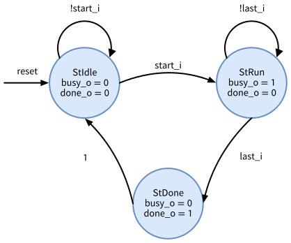
1 means always. The VHDL version names the states CTRL_IDLE, CTRL_RUN, and CTRL_DONE. The unused encoding 2'b11 of the SystemVerilog version, which also leads back to StIdle, is not drawn.
In VHDL, the controller looks as follows:
ctrl_fsm/vhdl/ctrl_fsm_ea.vhd
-- SPDX-FileCopyrightText: 2026 Simon Dorrer
-- SPDX-License-Identifier: Apache-2.0
-- Description: Moore FSM of a simple controller. A start_i pulse
-- moves it from idle to run (busy_o high) until last_i, then done_o
-- is high for one clock cycle before the FSM returns to idle.

library ieee;
use ieee.std_logic_1164.all;

entity ctrl_fsm is
  port(
    clk_i   : in  std_logic;
    rst_i   : in  std_logic;
    start_i : in  std_logic;
    last_i  : in  std_logic;
    busy_o  : out std_logic;
    done_o  : out std_logic
  );
end entity ctrl_fsm;

architecture rtl of ctrl_fsm is
  type t_state is (CTRL_IDLE, CTRL_RUN, CTRL_DONE);

  signal state      : t_state;
  signal next_state : t_state;
begin
  reg_proc: process(rst_i, clk_i) is
  begin
    if rst_i = '1' then
      state <= CTRL_IDLE;
    elsif rising_edge(clk_i) then
      state <= next_state;
    end if;
  end process reg_proc;

  fsm_logic: process(state, start_i, last_i) is
  begin
    next_state <= state;
    busy_o <= '0';
    done_o <= '0';
    case state is
      when CTRL_IDLE =>
        if start_i = '1' then
          next_state <= CTRL_RUN;
        end if;
      when CTRL_RUN =>
        busy_o <= '1';
        if last_i = '1' then
          next_state <= CTRL_DONE;
        end if;
      when CTRL_DONE =>
        done_o <= '1';
        next_state <= CTRL_IDLE;
    end case;
  end process fsm_logic;
end architecture rtl;
In SystemVerilog:
ctrl_fsm/rtl/ctrl_fsm.sv
// SPDX-FileCopyrightText: 2026 Simon Dorrer
// SPDX-License-Identifier: Apache-2.0
// Description: Moore FSM of a simple controller. A start_i pulse
// moves it from idle to run (busy_o high) until last_i, then done_o
// is high for one clock cycle before the FSM returns to idle.

`default_nettype none

module ctrl_fsm (
  input  logic clk_i,
  input  logic rst_ni,
  input  logic start_i,
  input  logic last_i,
  output logic busy_o,
  output logic done_o
);

  typedef enum logic [1:0] {
    StIdle,
    StRun,
    StDone
  } state_e;

  state_e state_d, state_q;

  // State register
  always_ff @(posedge clk_i or negedge rst_ni) begin
    if (!rst_ni) begin
      state_q <= StIdle;
    end else begin
      state_q <= state_d;
    end
  end

  // Next-state and output logic, defaults first
  always_comb begin
    state_d = state_q;
    busy_o  = 1'b0;
    done_o  = 1'b0;
    unique case (state_q)
      StIdle: begin
        if (start_i) state_d = StRun;
      end
      StRun: begin
        busy_o = 1'b1;
        if (last_i) state_d = StDone;
      end
      StDone: begin
        done_o  = 1'b1;
        state_d = StIdle;
      end
      default: state_d = StIdle;  // unused encoding 2'b11
    endcase
  end

endmodule

`default_nettype wire
- The state type is a
typedef enumwith an explicit base type (logic [1:0]). Following the lowRISC style guide, the type name ends in_eand the state names are UpperCamelCase with the prefixSt. - In VHDL, a
caseover an enumeration type with three values is complete. The 2-bit state of the SystemVerilog version has a fourth encoding,2'b11, which thedefaultitem sends back to idle. - As in VHDL, the next state defaults to the current state, and every output defaults to its inactive value before the
case. - The synthesis tool is free to choose the state encoding. Yosys 0.70 recognizes this FSM and re-encodes it one-hot, with three flip-flops instead of two.
- Write the transitions with
ifandelse. A conditional operator between enumeration values, such asstate_d = start_i ? StRun : StIdle;, is rejected by Icarus Verilog 14, which requires an explicit cast for it.
TipExercise: The Controller as a Mealy FSM
In a Mealy FSM, the outputs depend on the state and on the current inputs.
- The combinational process of the controller reads
start_iandlast_i. Why is the controller still a Moore FSM? - Change the controller into a Mealy FSM
ctrl_fsm_mealywith the same ports:done_ois high in the clock cycle in whichlast_iis high in the run state, and the FSM returns to idle at the next rising clock edge.busy_ostays high in the run state, as before. How many states do you need? Draw the state diagram, with the condition and the outputs on each arc (condition / busy_o done_o). - Implement
ctrl_fsm_mealyin the two-process style in VHDL (ctrl_fsm_mealy_ea.vhd) and in SystemVerilog (ctrl_fsm_mealy.sv), and lint the SystemVerilog version. - Number the clock cycles from 0, with the FSM idle in cycle 0.
start_iis high in cycle 0,last_iin cycle 3, and both are low otherwise. In which cycles arebusy_oanddone_ohigh in the Moore and in the Mealy version? What does the Mealy version gain, and what does itsdone_ocost?
Before continuing, please finish the previous exercise. Once you are done, compare with the solution below.
TipSolution: The Controller as a Mealy FSM
- The combinational process reads
start_iandlast_ionly in the conditions that choosestate_d.busy_oanddone_oare assigned in each state without any condition, so they depend only onstate_q. An output becomes a Mealy output as soon as it is assigned inside a condition on an input. - Two states are enough.
done_onow belongs to the transition fromStRunback toStIdle, in the clock cycle in whichlast_iis high, soStDoneis no longer needed. Figure 8 shows the state diagram.
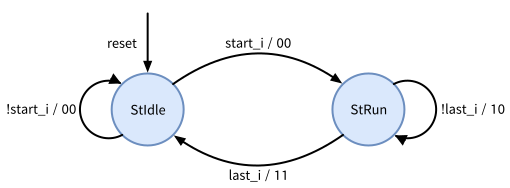
busy_o and done_o in the clock cycle in which the condition holds. done_o is high on the arc from StRun back to StIdle, in the same cycle as last_i.
- Compared with the Moore version, the state
StDonedisappears, so the enumeration needs only one bit, and in the run state the assignment todone_omoves into the condition onlast_i, which now returns to idle.
ctrl_fsm_mealy/vhdl/ctrl_fsm_mealy_ea.vhd
-- SPDX-FileCopyrightText: 2026 Simon Dorrer
-- SPDX-License-Identifier: Apache-2.0
-- Description: Mealy FSM of the simple controller. A start_i pulse
-- moves it from idle to run (busy_o high). done_o is high in the
-- clock cycle in which last_i is high, then the FSM returns to idle.

library ieee;
use ieee.std_logic_1164.all;

entity ctrl_fsm_mealy is
  port(
    clk_i   : in  std_logic;
    rst_i   : in  std_logic;
    start_i : in  std_logic;
    last_i  : in  std_logic;
    busy_o  : out std_logic;
    done_o  : out std_logic
  );
end entity ctrl_fsm_mealy;

architecture rtl of ctrl_fsm_mealy is
  type t_state is (CTRL_IDLE, CTRL_RUN);

  signal state      : t_state;
  signal next_state : t_state;
begin
  reg_proc: process(rst_i, clk_i) is
  begin
    if rst_i = '1' then
      state <= CTRL_IDLE;
    elsif rising_edge(clk_i) then
      state <= next_state;
    end if;
  end process reg_proc;

  fsm_logic: process(state, start_i, last_i) is
  begin
    next_state <= state;
    busy_o <= '0';
    done_o <= '0';
    case state is
      when CTRL_IDLE =>
        if start_i = '1' then
          next_state <= CTRL_RUN;
        end if;
      when CTRL_RUN =>
        busy_o <= '1';
        if last_i = '1' then
          done_o <= '1';  -- depends on an input: Mealy output
          next_state <= CTRL_IDLE;
        end if;
    end case;
  end process fsm_logic;
end architecture rtl;
ctrl_fsm_mealy/rtl/ctrl_fsm_mealy.sv
// SPDX-FileCopyrightText: 2026 Simon Dorrer
// SPDX-License-Identifier: Apache-2.0
// Description: Mealy FSM of the simple controller. A start_i pulse
// moves it from idle to run (busy_o high). done_o is high in the
// clock cycle in which last_i is high, then the FSM returns to idle.

`default_nettype none

module ctrl_fsm_mealy (
  input  logic clk_i,
  input  logic rst_ni,
  input  logic start_i,
  input  logic last_i,
  output logic busy_o,
  output logic done_o
);

  typedef enum logic {
    StIdle,
    StRun
  } state_e;

  state_e state_d, state_q;

  // State register
  always_ff @(posedge clk_i or negedge rst_ni) begin
    if (!rst_ni) begin
      state_q <= StIdle;
    end else begin
      state_q <= state_d;
    end
  end

  // Next-state and output logic, defaults first
  always_comb begin
    state_d = state_q;
    busy_o  = 1'b0;
    done_o  = 1'b0;
    unique case (state_q)
      StIdle: begin
        if (start_i) state_d = StRun;
      end
      StRun: begin
        busy_o = 1'b1;
        if (last_i) begin
          done_o  = 1'b1;  // depends on an input: Mealy output
          state_d = StIdle;
        end
      end
      default: state_d = StIdle;
    endcase
  end

endmodule

`default_nettype wire
The 1-bit state type of the SystemVerilog version has no unused encoding, and the default item stays only because the guidelines ask for unique case with a default (Section 2.9). Verilator reports no warning. Yosys 0.70 builds the Mealy controller from 4 cells with one flip-flop, against 9 cells with three flip-flops for the one-hot Moore version.
- Table 14 lists both versions cycle by cycle. Icarus Verilog, Verilator, and GHDL show exactly these values for the VHDL and the SystemVerilog versions (the check script of this chapter runs the sequence).
| Clock cycle | 0 | 1 | 2 | 3 | 4 | 5 |
|---|---|---|---|---|---|---|
start_i |
1 | 0 | 0 | 0 | 0 | 0 |
last_i |
0 | 0 | 0 | 1 | 0 | 0 |
| Moore state | StIdle |
StRun |
StRun |
StRun |
StDone |
StIdle |
Moore busy_o |
0 | 1 | 1 | 1 | 0 | 0 |
Moore done_o |
0 | 0 | 0 | 0 | 1 | 0 |
| Mealy state | StIdle |
StRun |
StRun |
StRun |
StIdle |
StIdle |
Mealy busy_o |
0 | 1 | 1 | 1 | 0 | 0 |
Mealy done_o |
0 | 0 | 0 | 1 | 0 | 0 |
The Mealy version raises done_o one clock cycle earlier, in the same cycle as last_i, needs one state less, and is ready for the next start one cycle earlier. The price is the combinational path from last_i to done_o. The output can glitch when last_i changes, and the path from the register that drives last_i, through this FSM, into the block that reads done_o must fit into one clock period. If that block also drives last_i combinationally from done_o, the two blocks even form a combinational loop. A Moore output comes directly from the state register and has none of these problems. If the earlier output is not needed, a register behind the Mealy output gives back the Moore timing.
2.5.10 Hierarchy and Generate
An instance of the adder of Section 2.5.1 with a width of 16 bits looks as follows in VHDL:
adder_0: entity work.adder
  generic map(
    WIDTH => 16
  )
  port map(
    a_i => x,
    b_i => y,
    sum_o => s
  );
And in SystemVerilog:
adder #(
  .WIDTH(16)
) adder_0 (
  .a_i  (x),
  .b_i  (y),
  .sum_o(s)
);
Always connect parameters and ports by name, never by position, and connect every port. Avoid the shortcuts .* and .name, which connect ports implicitly to signals of the same name and make the code hard to review.
A for loop outside a process is a generate loop, which creates hardware once per iteration:
gen_lane: for i in 0 to 3 generate
  adder_i: entity work.adder
    generic map(
      WIDTH => 8
    )
    port map(
      a_i => lane_a(i),
      b_i => lane_b(i),
      sum_o => lane_sum(i)
    );
end generate gen_lane;
logic [3:0][7:0] lane_a, lane_b;
logic [3:0][8:0] lane_sum;
for (genvar i = 0; i < 4; i++) begin : gen_lane
adder #(
.WIDTH(8)
) adder_i (
.a_i (lane_a[i]),
.b_i (lane_b[i]),
.sum_o(lane_sum[i])
);
endThe name of the block (gen_lane) becomes part of the hierarchical instance names, e.g., gen_lane[2].adder_i. Similarly, if (PARAM) begin : gen_name ... end outside a process creates hardware only if the parameter is true.
2.5.11 Packages, Typedefs, and Functions
A package collects constants, types, and functions that several modules share, like a VHDL package:
alu_pkg.sv
package alu_pkg;

  localparam int unsigned DATA_WIDTH = 8;

  typedef enum logic [1:0] {
    OpAdd,
    OpSub,
    OpAnd,
    OpOr
  } alu_op_e;

  typedef struct packed {
    alu_op_e               op;
    logic [DATA_WIDTH-1:0] operand;
  } instr_t;

  function automatic logic is_zero(input logic [DATA_WIDTH-1:0] data);
    is_zero = (data == '0);
  endfunction

endpackage
A module refers to the package contents with the scope operator ::, and the package file must be compiled before the modules that use it:
module alu (
  input  logic [alu_pkg::DATA_WIDTH-1:0] a_i,
  input  alu_pkg::instr_t                instr_i,
  output logic [alu_pkg::DATA_WIDTH-1:0] result_o,
  output logic                           zero_o
);

  always_comb begin
    unique case (instr_i.op)
      alu_pkg::OpAdd: result_o = a_i + instr_i.operand;
      alu_pkg::OpSub: result_o = a_i - instr_i.operand;
      alu_pkg::OpAnd: result_o = a_i & instr_i.operand;
      default:        result_o = a_i | instr_i.operand;
    endcase
  end

  assign zero_o = alu_pkg::is_zero(result_o);

endmodule- A
typedef struct packedreplaces a VHDL record. Its fields are accessed with a dot (instr_i.op), and the whole struct is also a plain bit vector, so it can be used as a port or stored in a register. - A
function automaticdescribes combinational logic, and every call becomes a separate copy of that logic. Declare functionsautomatic, so that every call gets its own variables. Tasks, which may contain timing, belong in testbenches.
ImportantTool Support for SystemVerilog Features
The default SystemVerilog front end of Yosys, which LibreLane uses unless USE_SLANG: True is set in its configuration, supports only part of the language. In Yosys 0.70, it fails on three constructs that Verilator and Icarus Verilog accept: import alu_pkg::* (the counterpart of use work.alu_pkg.all), return statements in functions, and unpacked arrays as ports. An import inside the module or its header gives a syntax error, and one before the module keyword gives a syntax error or an internal error. The code of this chapter therefore uses the scope operator pkg::NAME, assigns a function result to the function name, and uses packed arrays at ports. The slang front end of Yosys (read_slang, enabled in LibreLane with USE_SLANG: True) accepts all of these constructs. For the same reason, the counter of the AMS chip template uses `define macros instead of a package. When you use struct fields inside always_comb, Icarus Verilog prints a “sorry” message that the block becomes sensitive to the whole struct, which does not change the result.
2.5.12 What Is Synthesizable
Synthesis understands only a subset of SystemVerilog. Everything else is for simulation and testbenches only (Table 15).
| Synthesizable (RTL) | Simulation and testbenches only |
|---|---|
module, parameter, localparam, assign |
initial blocks (FPGA tools accept them for register initialization, ASICs have no initial values, use a reset) |
always_comb, always_ff, always_latch |
delays (#10), event waits inside procedural code (@(...), wait) |
if, case, for loops with constant bounds |
system tasks such as $display, $finish, $fatal, $dumpvars |
function automatic, generate loops and conditions |
=== and !==, real, string |
typedef enum, typedef struct packed, packed arrays, packages |
classes, randomize(), fork and join, tasks with timing |
+, -, *, shifts, comparisons on vectors |
loops whose number of iterations depends on data |
Be careful with / and %: they synthesize to large and slow logic unless the divisor is a constant power of two, in which case they reduce to a shift or a bit selection.
2.5.13 Verilog versus SystemVerilog
SystemVerilog grew out of Verilog. Verilog became the IEEE standard 1364 in 1995, was revised in 2001 and 2005, and was merged into SystemVerilog (IEEE 1800) in 2009. SystemVerilog is therefore a superset of Verilog: a Verilog file is also valid SystemVerilog, unless it uses one of the new keywords, such as logic or bit, as a name. In this course, you write SystemVerilog, but you will read plain Verilog all the time:
- Netlists. Yosys and LibreLane write their netlists in plain Verilog, e.g.,
final/nl/counter_top.nl.vof the counter macro in the AMS chip template: a port list in the style of Verilog-1995, a long list ofwires, and instances of standard cells such assg13cmos5l_dfrbpq_1. - Cell models. A gate-level simulation needs a simulation model of every standard cell. The models in the PDK (
sg13cmos5l_stdcell.v, with the user-defined primitives insg13cmos5l_udp.v) are written in Verilog with gate primitives, user-defined primitives, andspecifyblocks for the timing. - Generated code. All alternative HDLs of Section 2.3 emit Verilog or SystemVerilog.
- Existing code. Many open-source cores, older IP blocks, textbooks, and online examples are written in Verilog-2001, as is the Verilog cheat-sheet of Section 2.4. AI assistants often suggest code in the same style.
Table 16 maps the Verilog idioms you will meet onto the SystemVerilog of this chapter.
| Plain Verilog | SystemVerilog | Remark |
|---|---|---|
module m (a, y); followed by input a; and output y; |
module m (input logic a_i, output logic y_o); |
Verilog-1995 style, still used in netlists |
wire for assign and instance outputs, reg for always blocks |
logic for both |
the Verilog type depends on how a signal is assigned |
always @(a or b), since Verilog-2001 always @(*) |
always_comb |
complete sensitivity, latch check (Section 2.5.8) |
always @(posedge clk or negedge rst_n) |
always_ff @(posedge clk_i or negedge rst_ni) |
states the intent: flip-flops |
always @(*) that misses an assignment |
always_latch |
documents an intended latch |
parameter W = 8, `define |
parameter int unsigned W = 8, package |
typed constants, packages instead of global macros |
a localparam or `define per state |
typedef enum logic [1:0] {...} state_e |
assigning a plain number needs a cast (an error in Verilator and Icarus Verilog) |
slices of a wide vector, e.g., instr[9:8] |
typedef struct packed |
named fields, e.g., instr.op |
{W{1'b0}} |
'0 |
fills any width |
integer i; in the module, i = i + 1 |
for (int i = 0; i < N; i++) |
a loop variable local to the loop |
case with // synopsys full_case parallel_case |
unique case with default |
Yosys and Verilator read the comment, Icarus Verilog ignores it |
.v, read_verilog, iverilog |
.sv, read_verilog -sv, iverilog -g2012 |
Verilator reads both as SystemVerilog |
Most of these differences are syntax, but three of them matter beyond syntax:
regandwirefollow the assignment, not the hardware. In Verilog, a signal assigned in analwaysblock must be areg, even if it is combinational, and a signal driven by anassignor by an instance must be awire. If you turn anassigninto analwaysblock, you therefore have to change the declaration as well. In SystemVerilog, a variable (logicorreg) may be assigned in analwaysblock or by a singleassign, so the declaration stays the same, and no type name suggests a register that does not exist. Only awireassigned in analwaysblock remains an error (Icarus Verilog: not a valid l-value, Verilator:PROCASSWIREfor an internalwire).- The process types state the intent. For a missing assignment in
always @(*), Verilator and Yosys 0.70 only warn, and Yosys builds the latch. Foralways_comb, Yosys stops with an error (Section 2.5.8). - Checks belong in the language, not in comments. In Verilog, the comment
// synopsys full_case parallel_caseafter acasetells the synthesis tool that all missing values are don’t care (full_case) and that the items never overlap (parallel_case). Yosys reads it and builds no latch, and Verilator reads it as well: it drops theLATCHandCASEINCOMPLETEwarnings and stops the simulation when no item matches. Icarus Verilog ignores the comment and keeps the old value, so its simulation can differ from the netlist. Write a completecasewith adefaultitem instead, and adduniqueif the items are mutually exclusive. Keep thedefaultwithuniqueas well. Without it, Yosys handlesuniquelikefull_case: it silently takes the missing values as don’t care, even inalways_comb, and the netlist can differ from the simulation.
Most testbench features of this chapter are SystemVerilog as well, e.g., $fatal, $isunknown(), and int variables, and the verification part of the language (classes, randomization, assertions, and coverage) has no Verilog counterpart.
Finally, the tools must know which language they read. Verilator reads every file as SystemVerilog, also a .v file. Icarus Verilog reads Verilog-2005 unless you select SystemVerilog with -g2012, and the Yosys command read_verilog needs the option -sv, even for a file that ends in .sv. Name your files .sv, so that readers and editors know which language is inside.
TipExercise: Modernize a Verilog-2001 Module
The following priority encoder with registered outputs is written in plain Verilog-2001, as you find it in many older designs: idx is the index of the lowest set bit of req, and valid is high if any bit of req is set. Besides its old style, the module contains one mistake.
prio_enc/verilog/prio_enc.v
// SPDX-FileCopyrightText: 2026 Simon Dorrer
// SPDX-License-Identifier: Apache-2.0
// Description: Priority encoder with registered outputs in plain
// Verilog-2001. idx is the index of the lowest set bit of req,
// valid is high if any bit of req is set. This file contains a
// mistake on purpose (exercise), do not use it as a template.

module prio_enc (clk, rst_n, req, idx, valid);

  parameter N = 8;
  parameter W = 3;  // width of idx, must be log2(N)

  input          clk;
  input          rst_n;
  input  [N-1:0] req;
  output [W-1:0] idx;
  output         valid;

  reg    [W-1:0] idx;
  reg            valid;
  reg    [W-1:0] idx_next;
  wire           valid_next;
  integer        i;

  always @(posedge clk or negedge rst_n) begin
    if (!rst_n) begin
      idx   <= {W{1'b0}};
      valid <= 1'b0;
    end else begin
      idx   <= idx_next;
      valid <= valid_next;
    end
  end

  assign valid_next = |req;

  // The loop runs from the highest to the lowest bit, so the
  // lowest set bit is assigned last and wins.
  always @(*) begin
    for (i = N - 1; i >= 0; i = i - 1)
      if (req[i])
        idx_next = i;
  end

endmodule
- Which constructs are plain Verilog, and what are their SystemVerilog counterparts in Table 16?
- Save the file as
prio_enc.v, lint it withverilator --lint-only -Wall prio_enc.v, and synthesize it withyosys -p "read_verilog prio_enc.v; synth -top prio_enc; stat". What do the two tools report? - Translate the module into SystemVerilog in
prio_enc.sv, with the conventions of this chapter: ANSI ports with_iand_o,rst_ni,logic, and the two-process style with_dand_q. Do not fix the mistake yet. Synthesize your translation withread_verilog -sv. What has changed? - Fix the mistake and the remaining lint warning, and lint and synthesize the module again.
Before continuing, please finish the previous exercise. Once you are done, compare with the solution below.
TipSolution: Modernize a Verilog-2001 Module
- Each plain Verilog construct and its SystemVerilog counterpart:
- The port list with separate declarations (Verilog-1995 style) becomes an ANSI header with
logicports. - The
regs (the outputs andidx_next, assigned inalwaysblocks) and thewirevalid_next(driven by anassign) all becomelogic. always @(*)andalways @(posedge clk or negedge rst_n)becomealways_combandalways_ff.- The module-level
integer iwithi = i - 1becomesfor (int i = N - 1; i >= 0; i--). - The replication
{W{1'b0}}becomes'0. - The untyped parameters become
parameter int unsigned, andW, which must be set to matchNby hand, becomes$clog2(N). - The file extension
.vbecomes.sv.
- The port list with separate declarations (Verilog-1995 style) becomes an ANSI header with
- Verilator 5.052 reports two warnings.
WIDTHTRUNC: the 32-bitinteger iis assigned to the 3-bitidx_next.LATCH: if no bit ofreqis set, the loop assigns nothing, andidx_nextkeeps its old value. Yosys 0.70 only prints the warningLatch inferred for signal `\prio_enc.\idx_next'and builds 23 cells, among them four flip-flops$_DFF_PN0_foridxandvalidand three latches$_DLATCH_N_foridx_next. Leaving a value unassigned does not mean “don’t care” but “keep the old value.” - With
always_comb, Yosys stops withERROR: Latch inferred for signal `\prio_enc.\idx_d' from always_comb process. Verilator reports the sameLATCHwarning as before, andWIDTHTRUNCagain unless your translation already castsi. - The fix is a default assignment, as in every combinational process of this chapter:
prio_enc/rtl/prio_enc.sv
// SPDX-FileCopyrightText: 2026 Simon Dorrer
// SPDX-License-Identifier: Apache-2.0
// Description: Priority encoder with registered outputs. idx_o
// is the index of the lowest set bit of req_i, valid_o is high if
// any bit of req_i is set.

`default_nettype none

module prio_enc #(
  parameter int unsigned N = 8
) (
  input  logic                 clk_i,
  input  logic                 rst_ni,
  input  logic [N-1:0]         req_i,
  output logic [$clog2(N)-1:0] idx_o,
  output logic                 valid_o
);

  localparam int unsigned W = $clog2(N);

  logic [W-1:0] idx_d, idx_q;
  logic         valid_d, valid_q;

  // Register process: reset values and copies of the _d signals only
  always_ff @(posedge clk_i or negedge rst_ni) begin
    if (!rst_ni) begin
      idx_q   <= '0;
      valid_q <= 1'b0;
    end else begin
      idx_q   <= idx_d;
      valid_q <= valid_d;
    end
  end

  // Combinational process: defaults first, then all decisions
  always_comb begin
    idx_d   = '0;
    valid_d = |req_i;
    // The loop runs from the highest to the lowest bit, so the
    // lowest set bit is assigned last and wins.
    for (int i = N - 1; i >= 0; i--) begin
      if (req_i[i]) begin
        idx_d = W'(i);
      end
    end
  end

  assign idx_o   = idx_q;
  assign valid_o = valid_q;

endmodule

`default_nettype wire
- The width
Wfollows fromNwith$clog2(available since Verilog-2005), so it can no longer be set wrong. - The size cast
W'(i)makes the truncation of the loop variable explicit. - The loop variable is declared in the loop. It must be a signed
int: withint unsigned, the conditioni >= 0is always true. Verilator 5.052 reports a constant comparison (UNSIGNED) and an infinite loop (INFINITELOOP) and then stops with an internal error.
Verilator reports no warning, and Yosys builds 22 cells with the four flip-flops and no latch. While valid_o is low, idx_o is now 0, where the original kept the last index (or x before the first request). This does not matter, since idx_o is only meaningful while valid_o is high. The default idx_d = idx_q; would also be correct: it keeps the last index in the register, and Yosys turns the three idx flip-flops into flip-flops with enable ($_DFFE_PN0P_), again without a latch.
The testbench prio_enc/testbenches/verilog/prio_enc_tb.sv in the code folder applies all 256 values of req and compares the outputs with a reference model, checking idx_o only while valid_o is high. It also runs with your own translation, as long as it has the parameter N and the ports clk_i, rst_ni, req_i, idx_o, and valid_o. Copy it next to your translation, and run it:
T=/foss/designs/vlsi-design/content/sv_crashcourse/code/prio_enc
cp $T/testbenches/verilog/prio_enc_tb.sv .
iverilog -g2012 -o prio_enc_tb.vvp prio_enc.sv prio_enc_tb.sv
vvp prio_enc_tb.vvp
2.6 Testbenches
A testbench applies stimuli to the design under test (DUT) and checks its responses. It is simulation-only code, so it may use the whole language. Make every testbench self-checking: it compares the outputs with the expected values and reports a clear pass or fail, so that you never have to judge a waveform by eye to know whether a design works. Waveforms are for debugging. This section shows a SystemVerilog and a cocotb testbench for the tick generator of Section 2.5.7. Section 4 covers verification with cocotb in depth.
2.6.1 A SystemVerilog Testbench
tick_gen/testbenches/verilog/tick_gen_tb.sv
// SPDX-FileCopyrightText: 2026 Simon Dorrer
// SPDX-License-Identifier: Apache-2.0
// Description: Self-checking SystemVerilog testbench for tick_gen.

`timescale 1ns / 1ps

module tick_gen_tb;

  localparam int unsigned DIV           = 5;
  localparam real         CLK_PERIOD_NS = 20.0;  // 50 MHz

  logic clk   = 1'b0;
  logic rst_n = 1'b0;  // reset is active from time 0
  logic en    = 1'b0;
  logic tick;

  // Device under test (DUT)
  tick_gen #(
    .DIV(DIV)
  ) dut (
    .clk_i (clk),
    .rst_ni(rst_n),
    .en_i  (en),
    .tick_o(tick)
  );

  // Clock generation
  always #(CLK_PERIOD_NS / 2) clk = ~clk;

  // Stimulus and checks: inputs change and outputs are sampled on the
  // falling edge, so they never race with the DUT at the rising edge.
  initial begin
    $dumpfile("tick_gen_tb.vcd");
    $dumpvars(0, tick_gen_tb);

    repeat (2) @(negedge clk);
    rst_n = 1'b1;

    // Disabled: no tick at all
    repeat (3 * DIV) begin
      @(negedge clk);
      if (tick !== 1'b0) $fatal(1, "FAIL: tick while disabled");
    end

    // Enabled: exactly one tick every DIV clock cycles
    en = 1'b1;
    for (int cycle = 1; cycle <= 4 * DIV; cycle++) begin
      @(negedge clk);
      if (tick !== (cycle % DIV == 0)) begin
        $fatal(1, "FAIL: cycle %0d, tick = %b", cycle, tick);
      end
    end

    $display("PASS: tick_gen_tb");
    $finish;
  end

endmodule
`timescale 1ns / 1pssets the unit of the delays (#) and the precision of the simulation.- The testbench is a module without ports. It instantiates the DUT with a smaller
DIVthan the default, which keeps the simulation short. always #(CLK_PERIOD_NS / 2) clk = ~clk;generates the clock. Initial values in declarations are fine in a testbench.- The stimulus runs in an
initialblock. Inputs are changed and outputs are checked on the falling clock edge (@(negedge clk)), while the DUT acts on the rising edge. If the testbench and the DUT used the same edge, the result would depend on the order in which the simulator runs the processes, and Icarus Verilog and Verilator choose this order differently. - The checks use
!==, which also fails if the output isx, and end the simulation with$fatal(1, ...)on the first error. Do not use$errorfor this: Icarus Verilog only prints the message, reaches$finish, and exits with status 0, so a script or a make target cannot see that the test failed. $dumpfileand$dumpvarswrite all signals into a waveform file in the Value Change Dump (VCD) format, and$finishends the simulation.
2.6.2 A cocotb Testbench
cocotb (cocotb developers 2026) runs the testbench as Python code next to the simulator. Python then drives and reads the signals of the DUT through the programming interface of the simulator (the Verilog Procedural Interface, VPI, for Verilog simulators).
tick_gen/testbenches/cocotb/tick_gen_tb.py
# SPDX-FileCopyrightText: 2026 Simon Dorrer
# SPDX-License-Identifier: Apache-2.0
# Description: Self-checking cocotb testbench for tick_gen.

import os
from pathlib import Path

import cocotb
from cocotb.clock import Clock
from cocotb.triggers import ClockCycles, FallingEdge
from cocotb_tools.runner import get_results, get_runner

DIV = 5  # passed to the DUT as parameter in the runner below


async def start_up(dut):
    """Start a 50 MHz clock and reset the DUT for two cycles."""
    cocotb.start_soon(Clock(dut.clk_i, 20, "ns").start())
    dut.rst_ni.value = 0
    dut.en_i.value = 0
    await ClockCycles(dut.clk_i, 2)
    await FallingEdge(dut.clk_i)
    dut.rst_ni.value = 1


@cocotb.test()
async def test_no_tick_when_disabled(dut):
    """tick_o stays low while en_i is low."""
    await start_up(dut)
    for _ in range(3 * DIV):
        await FallingEdge(dut.clk_i)
        assert dut.tick_o.value == 0, "tick while disabled"


@cocotb.test()
async def test_tick_every_div_cycles(dut):
    """tick_o is high for one cycle every DIV cycles."""
    await start_up(dut)
    dut.en_i.value = 1
    for cycle in range(1, 4 * DIV + 1):
        await FallingEdge(dut.clk_i)
        expected = 1 if cycle % DIV == 0 else 0
        assert dut.tick_o.value == expected, \
            f"cycle {cycle}: expected {expected}, got {dut.tick_o.value}"


def tick_gen_runner():
    sim = os.getenv("SIM", "icarus")
    proj_path = Path(__file__).resolve().parent

    runner = get_runner(sim)
    runner.build(
        sources=[proj_path / "../../rtl/tick_gen.sv"],
        hdl_toplevel="tick_gen",
        parameters={"DIV": DIV},
        always=True,
        waves=True,
        timescale=("1ns", "1ps"),
    )
    results_xml = runner.test(
        hdl_toplevel="tick_gen",
        test_module="tick_gen_tb",
        waves=True,
    )

    # A failing test leaves the exit status at 0, so check the results
    num_tests, num_failed = get_results(results_xml)
    if num_failed:
        raise SystemExit(
            f"FAIL: {num_failed} of {num_tests} tests failed")


if __name__ == "__main__":
    tick_gen_runner()
- Every function decorated with
@cocotb.test()is a test. The tests of a file run one after another in the same simulation, so each one starts its own clock and applies the reset. - Tests are coroutines (
async def), which wait for simulator events withawait:RisingEdge(sig),FallingEdge(sig),ClockCycles(sig, n), orTimer(t, "ns"). As in the SystemVerilog testbench, inputs are driven and outputs are checked on the falling edge. dut.en_i.value = 1writes an input, anddut.tick_o.valuereads an output. A write takes effect at the end of the current time step, so reading the same signal right after writing it still returns the old value.cocotb.start_soon(Clock(dut.clk_i, 20, "ns").start())starts a 50 MHz clock that runs in parallel with the test.- A failing Python
assertfails the test, and the f-string message explains why. - The function
tick_gen_runner()follows the idiom of the AMS chip template: the file runs itself. It selects the simulator from the environment variableSIM(Icarus Verilog by default), builds the DUT with the given parameters, and runs the tests.runner.test()returns the path of the result fileresults.xml, but a failing test does not change the exit status ofpython3. The last lines therefore check the results withget_results()and exit with an error if any test failed.
2.6.3 SystemVerilog or cocotb?
Table 17 compares the two kinds of testbenches.
| Aspect | SystemVerilog testbench | cocotb testbench |
|---|---|---|
| Language | SystemVerilog (the full language, including the simulation subset) | Python 3 |
| Reference models | written in SystemVerilog | any Python code and library (e.g., NumPy) |
| Simulators | every SystemVerilog simulator | Icarus Verilog, Verilator, GHDL, and commercial simulators |
| DUT languages | SystemVerilog, VHDL only with a mixed-language simulator | the same testbench works for VHDL and SystemVerilog DUTs |
| Speed | fast, everything runs in the simulator | slower, every interaction passes through Python |
| In the AMS chip template | testbenches/verilog/ |
testbenches/cocotb/ |
In this course, we use both: a SystemVerilog testbench for a quick self-check of a block, and cocotb for everything that needs a reference model or randomized stimuli.
2.7 Linting, Simulation, and Synthesis in the IIC-OSIC-TOOLS Container
All tools you need are installed in the IIC-OSIC-TOOLS container (Section 1.9). In the AMS chip template, they are wrapped in make targets. In this chapter, you type the commands yourself, so that you know what is behind the targets when you use them later (Section 2.8).
2.7.1 Setting Up a Working Folder
Start the container (Section 1.13) and open a terminal on its desktop. Create a folder for the tick generator with the same structure as a macro of the AMS chip template:
mkdir -p /foss/designs/sv_exercises/tick_gen/{rtl,testbenches/verilog,testbenches/cocotb}
cd /foss/designs/sv_exercises/tick_gen
Save the three listings as rtl/tick_gen.sv, testbenches/verilog/tick_gen_tb.sv, and testbenches/cocotb/tick_gen_tb.py, e.g., with gedit, vim, or VS Code. With a local installation, /foss/designs is the folder ~/eda/designs on your laptop, so your files survive when the container is removed or updated. All commands of this section start in the folder /foss/designs/sv_exercises/tick_gen.
2.7.2 Linting with Verilator
A linter checks the code for errors and suspicious constructs without simulating it. Run it first, on every RTL file, after every change:
verilator --lint-only -Wall rtl/tick_gen.sv--lint-only only parses and checks the code, and -Wall enables all warnings, including the style warnings. Without any warning, Verilator only prints a short report and exits with status 0. Otherwise, it prints the warnings with file, line, and a link to their description, and exits with an error. Table 18 lists the warnings you will meet most often.
| Warning | Meaning | Typical fix |
|---|---|---|
IMPLICIT |
an undeclared name, Verilog created a 1-bit wire | fix the typo, add `default_nettype none |
UNDRIVEN, UNUSEDSIGNAL |
a signal is never assigned or never read | connect it or remove it |
WIDTHTRUNC, WIDTHEXPAND |
the widths of operands or of an assignment do not match | size the literals, extend with {1'b0, x}, or cast with N'(x) |
LATCH |
a combinational block (always_comb or always @(*)) does not assign a variable on every path |
default assignments first, complete case and else |
CASEINCOMPLETE |
a case does not cover all values |
add the missing items or a default |
BLKSEQ |
a blocking assignment = in always_ff |
use <= instead |
MULTIDRIVEN |
a variable is driven from more than one block | assign it in exactly one block |
DECLFILENAME |
the file name differs from the module name | one module per file, with the same name |
If a warning is a false alarm, you can switch it off for a few lines with /* verilator lint_off WIDTHEXPAND */ and /* verilator lint_on WIDTHEXPAND */, together with a comment that explains why. Never switch off warnings globally.
2.7.3 Simulating a SystemVerilog Testbench
Icarus Verilog compiles the design and the testbench into a simulation file, which vvp then runs:
iverilog -g2012 -o testbenches/verilog/tick_gen_tb.vvp \
  rtl/tick_gen.sv testbenches/verilog/tick_gen_tb.sv
cd testbenches/verilog
vvp tick_gen_tb.vvp
cd ../..
-g2012 selects the SystemVerilog standard IEEE 1800-2012, and -o names the output file. List the files in compile order: packages and files with `define macros first, then the modules. vvp writes the VCD file into the current folder, which is why we change into the testbench folder first and return afterwards. The simulation prints PASS: tick_gen_tb and exits with status 0, or stops at the first failed check with FATAL and exit status 1 (check it with echo $?).
Verilator can also run SystemVerilog testbenches. It compiles them into a C++ program, which is much faster for large designs. --binary builds an executable, and --timing enables the delays and event controls of the testbench. --timescale gives the RTL, which has no `timescale of its own, the same time unit as the testbench, and --trace enables the VCD output:
verilator --binary --timing --timescale 1ns/1ps --trace \
  --top-module tick_gen_tb -o tick_gen_tb \
  rtl/tick_gen.sv testbenches/verilog/tick_gen_tb.sv
cd testbenches/verilog
../../obj_dir/tick_gen_tb
cd ../..
2.7.4 Running a cocotb Testbench
A cocotb testbench in the template idiom runs itself:
cd testbenches/cocotb
python3 tick_gen_tb.py                  # with Icarus Verilog (default)
SIM=verilator python3 tick_gen_tb.py    # with Verilator
cd ../..
cocotb builds the simulation in the folder sim_build/, runs all tests, and prints a summary table with one line per test and a final line such as TESTS=2 PASS=2 FAIL=0 SKIP=0. The results are also stored in sim_build/results.xml. With Icarus Verilog, the waveform is written to sim_build/tick_gen.fst, with Verilator to sim_build/dump.vcd.
2.7.5 Viewing Waveforms
Open a waveform with GTKWave or Surfer:
gtkwave testbenches/verilog/tick_gen_tb.vcd
surfer testbenches/cocotb/sim_build/tick_gen.fst
In GTKWave, select a module in the hierarchy on the left, append its signals to the wave window, and zoom to fit. GTKWave can store the selected signals in a save file (.gtkw), which you pass as a second argument the next time, e.g., gtkwave tick_gen_tb.vcd tick_gen_tb.gtkw in the testbench folder. The AMS chip template keeps such save files next to its testbenches.
2.7.6 A Quick Synthesis Check with Yosys
A simulation shows what a design does, but not which hardware it becomes. A quick synthesis with Yosys answers this in a second:
yosys -p "read_verilog -sv rtl/tick_gen.sv; synth -top tick_gen; stat"read_verilog -sv reads the file with the SystemVerilog front end, synth -top tick_gen synthesizes the design with tick_gen as top module onto generic gates, and stat prints the cell statistics at the end of the log. Check that the number of flip-flops ($_DFF_* and $_DFFE_* cells) matches the registers you intended and that there are no latches ($_DLATCH_* cells). The letters of a flip-flop name give the clock edge, the reset polarity, the reset value, and the enable polarity: $_DFFE_PN0P_ is a flip-flop on the positive clock edge (P) with an active-low reset (N) to zero (0) and an active-high enable (P). In the LibreLane flow, Yosys maps these generic cells onto the standard cells of SG13CMOS5L (Section 5).
TipExercise: Lint, Simulate, and Synthesize the Tick Generator
- Set up the folder as described in Section 2.7.1 and save the three listings of the tick generator.
- Lint the RTL with Verilator.
- Run the SystemVerilog testbench with Icarus Verilog and look at the waveform in GTKWave. Find the cycles in which
tickis high and compare them withcount_qinside the DUT. - Run the cocotb testbench with Icarus Verilog and with Verilator, and open the cocotb waveform in Surfer.
- Synthesize the RTL with Yosys. How many cells and flip-flops does it need, and of which types are the flip-flops?
- Change
DIVto 8 in both testbenches and rerun them. Since 8 is a power of two, the 3-bit counter uses all eight of its values. Then build in a bug: comparecount_qwithCOUNT_LAST - 1instead ofCOUNT_LAST. Do both testbenches catch it?
Before continuing, please finish the previous exercise. Once you are done, compare with the solution below.
TipSolution: Lint, Simulate, and Synthesize the Tick Generator
- Verilator reports no warning.
- The simulation prints
PASS: tick_gen_tb. WithDIV = 5,tickis high in the clock cycle aftercount_qhas reached 4, i.e., once every five cycles whileenis high. - Both runs end with
TESTS=2 PASS=2 FAIL=0 SKIP=0. Icarus Verilog writessim_build/tick_gen.fst, Verilatorsim_build/dump.vcd. - With the default
DIV = 10, Yosys 0.70 reports 17 cells, among them five flip-flops: four$_DFFE_PN0P_cells forcount_q(with an active-high enable input, which comes fromen_i) and one$_DFF_PN0_cell fortick_q. - With
DIV = 8, both testbenches pass. With the bug, the counter wraps one cycle early, and both testbenches fail: the SystemVerilog testbench stops withFATALand exit status 1, cocotb reportsFAILfortest_tick_every_div_cycles, and the runner exits with an error.
TipExercise: PWM Generator with a SystemVerilog Testbench
Design a pulse-width modulation (PWM) generator pwm in the two-process style with these properties:
- A parameter
WIDTH(default 8) and the portsclk_i,rst_ni(asynchronous, active low),duty_i(WIDTHbits), andpwm_o. - An internal counter counts from 0 to \(2^\mathrm{WIDTH}-1\) and wraps around, so one PWM period lasts \(2^\mathrm{WIDTH}\) clock cycles.
- In every period,
pwm_ois high for exactlyduty_iclock cycles.duty_i = 0keeps the output low, and the maximum duty cycle is \((2^\mathrm{WIDTH}-1)/2^\mathrm{WIDTH}\). pwm_ocomes directly from a flip-flop, so that it has no glitches on its way to a pad.
- Write the RTL in
pwm/rtl/pwm.svand lint it. - Write a self-checking SystemVerilog testbench
pwm/testbenches/verilog/pwm_tb.svwithWIDTH = 4. For every one of the 16 duty values, it counts the high cycles ofpwm_owithin one period and stops with$fatalif the count is wrong. Also check thatpwm_ois neverx. - Run the testbench with Icarus Verilog and inspect the waveform.
Before continuing, please finish the previous exercise. Once you are done, compare with the solution below.
TipSolution: PWM Generator with a SystemVerilog Testbench
pwm/rtl/pwm.sv
// SPDX-FileCopyrightText: 2026 Simon Dorrer
// SPDX-License-Identifier: Apache-2.0
// Description: PWM generator. In every period of 2**WIDTH clock
// cycles, pwm_o is high for exactly duty_i cycles (duty_i = 0 keeps
// it low).

`default_nettype none

module pwm #(
  parameter int unsigned WIDTH = 8
) (
  input  logic             clk_i,
  input  logic             rst_ni,
  input  logic [WIDTH-1:0] duty_i,
  output logic             pwm_o
);

  logic [WIDTH-1:0] count_d, count_q;
  logic             pwm_d, pwm_q;

  always_ff @(posedge clk_i or negedge rst_ni) begin
    if (!rst_ni) begin
      count_q <= '0;
      pwm_q   <= 1'b0;
    end else begin
      count_q <= count_d;
      pwm_q   <= pwm_d;
    end
  end

  always_comb begin
    count_d = count_q + 1'b1;  // wraps from 2**WIDTH - 1 to 0
    pwm_d   = (count_q < duty_i);
  end

  // Registered output: no glitches on the way to a pad
  assign pwm_o = pwm_q;

endmodule

`default_nettype wire
Since the counter has exactly WIDTH bits, it wraps around without any compare logic. The output register delays pwm_o by one cycle with respect to the comparison, which does not change the number of high cycles per period.
pwm/testbenches/verilog/pwm_tb.sv
// SPDX-FileCopyrightText: 2026 Simon Dorrer
// SPDX-License-Identifier: Apache-2.0
// Description: Self-checking SystemVerilog testbench for pwm,
// testing all duty values of a 4-bit PWM.

`timescale 1ns / 1ps

module pwm_tb;

  localparam int unsigned WIDTH         = 4;
  localparam int unsigned PERIOD        = 2 ** WIDTH;
  localparam real         CLK_PERIOD_NS = 20.0;  // 50 MHz

  logic             clk   = 1'b0;
  logic             rst_n = 1'b0;
  logic [WIDTH-1:0] duty  = '0;
  logic             pwm_out;
  int unsigned      high_cycles;

  pwm #(
    .WIDTH(WIDTH)
  ) dut (
    .clk_i (clk),
    .rst_ni(rst_n),
    .duty_i(duty),
    .pwm_o (pwm_out)
  );

  always #(CLK_PERIOD_NS / 2) clk = ~clk;

  initial begin
    $dumpfile("pwm_tb.vcd");
    $dumpvars(0, pwm_tb);

    repeat (2) @(negedge clk);
    rst_n = 1'b1;

    for (int d = 0; d < PERIOD; d++) begin
      duty = WIDTH'(d);
      repeat (2) @(negedge clk);  // the new duty reaches pwm_o

      // Any PERIOD consecutive cycles contain exactly d high cycles
      high_cycles = 0;
      repeat (PERIOD) begin
        @(negedge clk);
        if ($isunknown(pwm_out)) $fatal(1, "FAIL: pwm_o is X or Z");
        if (pwm_out) high_cycles++;
      end
      if (high_cycles != d) begin
        $fatal(1, "FAIL: duty %0d gives %0d high cycles", d,
               high_cycles);
      end
    end

    $display("PASS: pwm_tb");
    $finish;
  end

endmodule
After a new duty value is applied, the testbench waits two cycles until it has reached the output register. Then any \(2^\mathrm{WIDTH}\) consecutive cycles contain exactly duty high cycles, regardless of where the period starts, so the testbench does not need to know the internal counter. $isunknown() is true if any bit is x or z. The commands are:
cd /foss/designs/sv_exercises/pwm
verilator --lint-only -Wall rtl/pwm.sv
iverilog -g2012 -o testbenches/verilog/pwm_tb.vvp rtl/pwm.sv testbenches/verilog/pwm_tb.sv
cd testbenches/verilog && vvp pwm_tb.vvp
gtkwave pwm_tb.vcd
To check that the testbench really checks something, change < to <= in the comparison: the testbench then stops with FATAL and the message FAIL: duty 0 gives 1 high cycles.
TipExercise: PWM Generator with a cocotb Testbench
Write a cocotb testbench pwm/testbenches/cocotb/pwm_tb.py for your PWM generator from the previous exercise, again with WIDTH = 4:
- A test
test_all_duty_valueswith the same check as the SystemVerilog testbench. In cocotb,dut.pwm_o.value.is_resolvableis false if any bit isxorz, sonot dut.pwm_o.value.is_resolvablecorresponds to$isunknown(). - A test
test_against_modelthat changesduty_ito random values at random times (use a fixed seed, e.g.,random.Random(42)) and comparespwm_oin every clock cycle with a cycle-accurate Python model of the counter and the output register. - A runner in the template idiom of Section 2.6.2, which exits with an error if a test fails.
Run the testbench with Icarus Verilog and with Verilator.
Before continuing, please finish the previous exercise. Once you are done, compare with the solution below.
TipSolution: PWM Generator with a cocotb Testbench
pwm/testbenches/cocotb/pwm_tb.py
# SPDX-FileCopyrightText: 2026 Simon Dorrer
# SPDX-License-Identifier: Apache-2.0
# Description: Self-checking cocotb testbench for pwm (4-bit PWM).

import os
import random
from pathlib import Path

import cocotb
from cocotb.clock import Clock
from cocotb.triggers import ClockCycles, FallingEdge
from cocotb_tools.runner import get_results, get_runner

WIDTH = 4
PERIOD = 2**WIDTH


async def start_up(dut):
    """Start a 50 MHz clock and reset the DUT for two cycles."""
    cocotb.start_soon(Clock(dut.clk_i, 20, "ns").start())
    dut.rst_ni.value = 0
    dut.duty_i.value = 0
    await ClockCycles(dut.clk_i, 2)
    await FallingEdge(dut.clk_i)
    dut.rst_ni.value = 1


@cocotb.test()
async def test_all_duty_values(dut):
    """For every duty d, pwm_o is high for d cycles per period."""
    await start_up(dut)
    for duty in range(PERIOD):
        dut.duty_i.value = duty
        for _ in range(2):  # the new duty reaches pwm_o
            await FallingEdge(dut.clk_i)
        high_cycles = 0
        for _ in range(PERIOD):
            await FallingEdge(dut.clk_i)
            assert dut.pwm_o.value.is_resolvable, "pwm_o is X or Z"
            high_cycles += int(dut.pwm_o.value)
        assert high_cycles == duty, \
            f"duty {duty} gives {high_cycles} high cycles"


@cocotb.test()
async def test_against_model(dut):
    """Random duty changes, checked cycle by cycle against a model."""
    await start_up(dut)
    rng = random.Random(42)  # fixed seed: every run is reproducible
    count, pwm, duty = 0, 0, 0  # model state after reset
    for _ in range(20 * PERIOD):
        if rng.random() < 0.05:
            # Keep the value in Python: a write becomes visible in
            # the DUT only at the end of the current time step
            duty = rng.randrange(PERIOD)
            dut.duty_i.value = duty
        await FallingEdge(dut.clk_i)
        # Model of the rising edge: both registers update at once
        pwm = 1 if count < duty else 0
        count = (count + 1) % PERIOD
        assert dut.pwm_o.value == pwm, \
            f"expected {pwm}, got {dut.pwm_o.value}"


def pwm_runner():
    sim = os.getenv("SIM", "icarus")
    proj_path = Path(__file__).resolve().parent

    runner = get_runner(sim)
    runner.build(
        sources=[proj_path / "../../rtl/pwm.sv"],
        hdl_toplevel="pwm",
        parameters={"WIDTH": WIDTH},
        always=True,
        waves=True,
        timescale=("1ns", "1ps"),
    )
    results_xml = runner.test(
        hdl_toplevel="pwm",
        test_module="pwm_tb",
        waves=True,
    )

    # A failing test leaves the exit status at 0, so check the results
    num_tests, num_failed = get_results(results_xml)
    if num_failed:
        raise SystemExit(
            f"FAIL: {num_failed} of {num_tests} tests failed")


if __name__ == "__main__":
    pwm_runner()
The model in test_against_model mirrors the two registers of the DUT: at every rising edge, the new pwm value is computed from the old counter value, and the counter increments, exactly like the two non-blocking assignments in always_ff. The comment on duty explains why the model keeps its own copy of the value it writes. Reading dut.duty_i.value right after the write would still return the old value, and the model would be one cycle off. Both simulators report TESTS=2 PASS=2 FAIL=0 SKIP=0. The model test is the stronger one: a counter that wraps at 14 instead of 15 fails both tests, but only the model test would also find a bug that keeps the number of high cycles right and shifts the pulse within the period.
TipExercise: Sequence Detector FSM
The following VHDL FSM detects the bit pattern 1011 in a serial input. It samples one bit at each rising clock edge, and overlapping occurrences count, so 1011011 contains the pattern twice. detect_o is high for one clock cycle after the edge that sampled the last 1 of the pattern (Moore output).
seq_detect/vhdl/seq_detect_ea.vhd
-- SPDX-FileCopyrightText: 2026 Simon Dorrer
-- SPDX-License-Identifier: Apache-2.0
-- Description: Moore FSM that detects the bit pattern 1011 in the
-- serial input bit_i (one bit per rising clock edge, overlapping
-- occurrences count). detect_o is high for one cycle after the edge
-- that sampled the last 1.

library ieee;
use ieee.std_logic_1164.all;

entity seq_detect is
  port(
    clk_i    : in  std_logic;
    rst_i    : in  std_logic;
    bit_i    : in  std_logic;
    detect_o : out std_logic
  );
end entity seq_detect;

architecture rtl of seq_detect is
  -- Each state names the longest matched prefix of 1011
  type t_state is (DET_IDLE, DET_1, DET_10, DET_101, DET_1011);

  signal state      : t_state;
  signal next_state : t_state;
begin
  reg_proc: process(rst_i, clk_i) is
  begin
    if rst_i = '1' then
      state <= DET_IDLE;
    elsif rising_edge(clk_i) then
      state <= next_state;
    end if;
  end process reg_proc;

  fsm_logic: process(state, bit_i) is
  begin
    next_state <= state;
    detect_o <= '0';
    case state is
      when DET_IDLE =>
        if bit_i = '1' then
          next_state <= DET_1;
        end if;
      when DET_1 =>
        if bit_i = '0' then
          next_state <= DET_10;
        end if;
      when DET_10 =>
        if bit_i = '1' then
          next_state <= DET_101;
        else
          next_state <= DET_IDLE;
        end if;
      when DET_101 =>
        if bit_i = '1' then
          next_state <= DET_1011;
        else
          next_state <= DET_10;
        end if;
      when DET_1011 =>
        detect_o <= '1';
        if bit_i = '1' then
          next_state <= DET_1;
        else
          next_state <= DET_10;
        end if;
    end case;
  end process fsm_logic;
end architecture rtl;
- Draw the state diagram.
- Translate the FSM into a SystemVerilog module
seq_detectinseq_detect/rtl/seq_detect.sv, with an asynchronous active-low resetrst_niinstead ofrst_iand otherwise the same port names, which the testbench below uses. Lint it. - Verify it with the following cocotb testbench, which compares
detect_owith a Python reference model for a directed and a random bit stream. Run it with Icarus Verilog and with Verilator.
seq_detect/testbenches/cocotb/seq_detect_tb.py
# SPDX-FileCopyrightText: 2026 Simon Dorrer
# SPDX-License-Identifier: Apache-2.0
# Description: Self-checking cocotb testbench for seq_detect with a
# Python reference model.

import os
import random
from pathlib import Path

import cocotb
from cocotb.clock import Clock
from cocotb.triggers import ClockCycles, FallingEdge
from cocotb_tools.runner import get_results, get_runner

PATTERN = [1, 0, 1, 1]


async def start_up(dut):
    """Start a 50 MHz clock and reset the DUT for two cycles."""
    cocotb.start_soon(Clock(dut.clk_i, 20, "ns").start())
    dut.rst_ni.value = 0
    dut.bit_i.value = 0
    await ClockCycles(dut.clk_i, 2)
    await FallingEdge(dut.clk_i)
    dut.rst_ni.value = 1


async def send_and_check(dut, bits):
    """Send one bit per cycle, compare detect_o with the model."""
    history = []
    detections = 0
    for bit in bits:
        dut.bit_i.value = bit
        # The DUT samples the bit at the rising edge in between
        await FallingEdge(dut.clk_i)
        history.append(bit)
        expected = 1 if history[-len(PATTERN):] == PATTERN else 0
        assert dut.detect_o.value == expected, \
            f"after bits ...{history[-8:]}: " \
            f"expected {expected}, got {dut.detect_o.value}"
        detections += expected
    return detections


@cocotb.test()
async def test_overlapping(dut):
    """1011011 contains the pattern twice, the second overlapping."""
    await start_up(dut)
    detections = await send_and_check(dut, [1, 0, 1, 1, 0, 1, 1, 0, 0])
    assert detections == 2, f"expected 2 detections, got {detections}"


@cocotb.test()
async def test_random_bits(dut):
    """A long random bit stream against the reference model."""
    await start_up(dut)
    rng = random.Random(1234)  # fixed seed: every run is reproducible
    bits = [rng.randint(0, 1) for _ in range(500)]
    detections = await send_and_check(dut, bits)
    # Guard against a test that passes without ever seeing the pattern
    assert detections > 0, "no pattern in the random stream"
    dut._log.info(f"{detections} detections in {len(bits)} bits")


def seq_detect_runner():
    sim = os.getenv("SIM", "icarus")
    proj_path = Path(__file__).resolve().parent

    runner = get_runner(sim)
    runner.build(
        sources=[proj_path / "../../rtl/seq_detect.sv"],
        hdl_toplevel="seq_detect",
        always=True,
        waves=True,
        timescale=("1ns", "1ps"),
    )
    results_xml = runner.test(
        hdl_toplevel="seq_detect",
        test_module="seq_detect_tb",
        waves=True,
    )

    # A failing test leaves the exit status at 0, so check the results
    num_tests, num_failed = get_results(results_xml)
    if num_failed:
        raise SystemExit(
            f"FAIL: {num_failed} of {num_tests} tests failed")


if __name__ == "__main__":
    seq_detect_runner()
Before continuing, please finish the previous exercise. Once you are done, compare with the solution below.
TipSolution: Sequence Detector FSM
Each state stores the longest prefix of 1011 that the received bits end with. A 0 after 1011 leaves 10, and a 1 leaves 1, which is how overlapping occurrences are detected. Table 19 gives the state diagram as a table, with the state names of the VHDL version. In the SystemVerilog solution, DET_IDLE becomes StIdle, DET_1 becomes St1, and so on.
| State | Next state for bit_i = 0 |
Next state for bit_i = 1 |
detect_o |
|---|---|---|---|
DET_IDLE |
DET_IDLE |
DET_1 |
0 |
DET_1 |
DET_10 |
DET_1 |
0 |
DET_10 |
DET_IDLE |
DET_101 |
0 |
DET_101 |
DET_10 |
DET_1011 |
0 |
DET_1011 |
DET_10 |
DET_1 |
1 |
seq_detect/rtl/seq_detect.sv
// SPDX-FileCopyrightText: 2026 Simon Dorrer
// SPDX-License-Identifier: Apache-2.0
// Description: Moore FSM that detects the bit pattern 1011 in the
// serial input bit_i (one bit per rising clock edge, overlapping
// occurrences count). detect_o is high for one cycle after the edge
// that sampled the last 1.

`default_nettype none

module seq_detect (
  input  logic clk_i,
  input  logic rst_ni,
  input  logic bit_i,
  output logic detect_o
);

  // Each state names the longest matched prefix of 1011
  typedef enum logic [2:0] {
    StIdle,
    St1,
    St10,
    St101,
    St1011
  } state_e;

  state_e state_d, state_q;

  always_ff @(posedge clk_i or negedge rst_ni) begin
    if (!rst_ni) begin
      state_q <= StIdle;
    end else begin
      state_q <= state_d;
    end
  end

  always_comb begin
    state_d  = state_q;
    detect_o = 1'b0;
    unique case (state_q)
      StIdle: begin
        if (bit_i) state_d = St1;
      end
      St1: begin
        if (!bit_i) state_d = St10;
      end
      St10: begin
        if (bit_i) state_d = St101;
        else       state_d = StIdle;
      end
      St101: begin
        if (bit_i) state_d = St1011;
        else       state_d = St10;
      end
      St1011: begin
        detect_o = 1'b1;
        if (bit_i) state_d = St1;
        else       state_d = St10;
      end
      default: state_d = StIdle;  // unused encodings
    endcase
  end

endmodule

`default_nettype wire
Five states need a 3-bit encoding, so three encodings are unused, and the default item sends them back to idle. Both simulators report TESTS=2 PASS=2 FAIL=0 SKIP=0, and the random stream of 500 bits contains the pattern 31 times. The testbench checks that this count is not zero, so that the random test cannot pass without ever seeing the pattern. Icarus Verilog prints a “sorry” message that it ignores unique, which you can disregard. Since cocotb is independent of the HDL, the same testbench also runs the VHDL version with GHDL (with the active-high reset rst_i instead of rst_ni), and both versions pass.
2.8 Hands-On: The Counter of the AMS Chip Template
In this course, you use the SG13CMOS5L version of the AMS chip template, ihp-sg13cmos5l-ams-chip-template, together with its tutorial. Its digital example is the macro macros/counter: an 8-bit counter with a synchronous reset, an enable, and a wrap-around at CTR_MAX, plus a wrapper counter_top, which converts the active-low reset of the chip into the active-high reset of the counter. The tutorial shows the complete code of the counter in its section counter.sv. The macro comes with a SystemVerilog and a cocotb testbench, and its Makefile wraps the commands of Section 2.7 into make targets. In the following exercises, you first type the commands yourself and only then look at the targets.
TipExercise: Lint and Simulate the Counter by Hand
Clone the template into your designs folder (if you have not done so yet) and change into the counter macro:
cd /foss/designs
git clone https://github.com/iic-jku/ihp-sg13cmos5l-ams-chip-template.git
cd ihp-sg13cmos5l-ams-chip-template/macros/counter- Read
rtl/constants.sv,rtl/counter.sv, andrtl/counter_top.sv. - Lint
counter_toptogether with the files it needs withverilator --lint-only -Wall. In which order do you have to pass the files, and why? - Compile the SystemVerilog testbench
testbenches/verilog/counter_top_tb.svwith Icarus Verilog, run it in its folder, and open the waveform with the saved signal listcounter_top_tb.gtkw. - Run the cocotb testbench
testbenches/cocotb/counter_top_tb.pywith the default simulator and open its waveform. - The counter has four behaviors: reset, hold while disabled, increment while enabled, and wrap-around at
CTR_MAX. Which of them does each testbench actually check?
Before continuing, please finish the previous exercise. Once you are done, compare with the solution below.
TipSolution: Lint and Simulate the Counter by Hand
# Lint (no warning, even with -Wall)
verilator --lint-only -Wall rtl/constants.sv rtl/counter.sv rtl/counter_top.sv

# SystemVerilog testbench with Icarus Verilog
iverilog -g2012 -o testbenches/verilog/counter_top_tb.vvp \
  rtl/constants.sv rtl/counter.sv rtl/counter_top.sv \
  testbenches/verilog/counter_top_tb.sv
cd testbenches/verilog
vvp counter_top_tb.vvp
gtkwave counter_top_tb.vcd counter_top_tb.gtkw

# cocotb testbench
cd ../cocotb
python3 counter_top_tb.py
gtkwave sim_build/counter_top.fst counter_top_tb.gtkwconstants.svdefines the macros`COUNTER_MAX_DEFAULTand`CLK_FREQ_DEFAULT, whichcounter_top.svand the testbench use. A macro must be defined before it is used, and the tools read the files in the given order, soconstants.svcomes first.- The SystemVerilog testbench prints
PASS: simulation complete., and the cocotb testbench reportsTESTS=4 PASS=4 FAIL=0 SKIP=0. - The cocotb testbench checks all four behaviors, one test each. The SystemVerilog testbench (template version of October 2026) checks only two: the counter is zero after the reset, and it stays zero while disabled. It enables the counter for a full wrap-around, but does not check the values, so increment and wrap-around are only visible in the waveform. A
PASSonly means that the implemented checks passed.
TipExercise: The Counter in the Two-Process Style
- Draw the counter as a synchronous sequential circuit in the structure of Figure 4. Which signal is the state, which are the inputs, and which operations does the next-state logic need?
- Turn your diagram into the two-process style: rewrite
rtl/counter.svwithcount_dandcount_q, the register inalways_ffand the next-state logic inalways_comb. Keep the module name, the parameters, the ports, and the behavior (synchronous reset, enable, wrap-around atCTR_MAX) exactly as they are. - Lint the design and run both testbenches again. All checks must still pass, which shows that your refactoring did not change the checked behavior.
- Now build in a bug: let the counter wrap one value early (compare with
CTR_MAX - 1). Run both testbenches again and check their exit status withecho $?. Which testbench finds the bug? What does the exit status tell you? - Restore the original file with
git restore rtl/counter.sv.
Before continuing, please finish the previous exercise. Once you are done, compare with the solution below.
TipSolution: The Counter in the Two-Process Style
Figure 9 shows the counter in the structure of Figure 4. The state is count_q, held in CTR_BW flip-flops with the clock clock_i and the synchronous reset reset_i. The next-state logic gets count_q and the input enable_i and needs four parts: a comparator with CTR_MAX, an incrementer, a first multiplexer that selects zero at the wrap-around, and a second multiplexer that keeps count_q while enable_i is low.
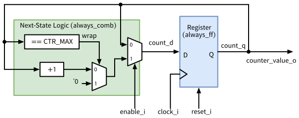
count_q and has the synchronous reset reset_i. In the next-state logic, the comparator and the incrementer work on count_q in parallel, the first multiplexer selects zero at the wrap-around, and the second keeps count_q while enable_i is low.
In the code, the register becomes always_ff, and the next-state logic becomes always_comb, where the two multiplexers turn into the if and else decisions:
macros/counter/rtl/counter.sv (two-process version)
// SPDX-FileCopyrightText: 2026 Simon Dorrer and Harald Pretl
// SPDX-License-Identifier: Apache-2.0 WITH SHL-2.1
// Description: This file implements an N-bit up counter with
// synchronous reset & enable in SystemVerilog (two-process style).

`default_nettype none
`ifndef __COUNTER__
`define __COUNTER__

module counter #(
  parameter int unsigned       CTR_BW  = 8,
  parameter logic [CTR_BW-1:0] CTR_MAX = 2**CTR_BW - 1
)(
  input logic               clock_i,
  input logic               reset_i,
  input logic               enable_i,

  output logic [CTR_BW-1:0] counter_value_o
);

  logic [CTR_BW-1:0] count_d, count_q;

  // Register process: synchronous reset and copy of count_d only
  always_ff @(posedge clock_i) begin
    if (reset_i) begin
      count_q <= '0;
    end else begin
      count_q <= count_d;
    end
  end

  // Combinational process: next counter value, wraps around at CTR_MAX
  always_comb begin
    count_d = count_q;
    if (enable_i) begin
      if (count_q == CTR_MAX) begin
        count_d = '0;
      end else begin
        count_d = count_q + 1'b1;
      end
    end
  end

  assign counter_value_o = count_q;

endmodule // counter

`endif
`default_nettype wire
The synchronous reset stays in the register process, so always_ff holds the reset value and the copy of count_d, as in your VHDL reg_proc. Putting the reset into the combinational process as the first decision would describe the same hardware. Lint and both testbenches pass as before.
With the bug, the SystemVerilog testbench still prints PASS and exits with status 0, because it does not check the wrap-around. In the cocotb testbench, test_wraps_at_max fails, but python3 counter_top_tb.py still exits with status 0, because the runner of the template does not evaluate results.xml (compare it with the runner of Section 2.6.2). Two lessons follow: a testbench is only as good as its checks, and an exit status is only useful if the script sets it. Both matter as soon as testbenches run automatically, e.g., in a regression with make or in continuous integration.
TipExercise: What Is Behind the Make Targets?
Open macros/counter/Makefile of the template.
make helplists all targets. Try it, then trymake -n sim-rtl-verilog, which prints the commands of a target without running them (dry run). What does the Makefile check before it runs a target, and what do you have to do if this check fails?- Find the targets that run the commands you typed in the previous exercises, and compare their commands (
make -n <target>) with yours. What is different?
Before continuing, please finish the previous exercise. Once you are done, compare with the solution below.
TipSolution: What Is Behind the Make Targets?
Every target except help and clean first checks that the environment variable PDK is ihp-sg13cmos5l, because the macro is built for this PDK. If the shell is set to another PDK (the default of the container is ihp-sg13g2, check it with echo $PDK), the Makefile stops with an error message, even for a dry run. Switch the PDK with sak-pdk ihp-sg13cmos5l in the same shell and try again. Your own commands did not need this, because an RTL simulation does not use the PDK. Table 20 compares the targets with your commands.
| Your command | Make target | Differences |
|---|---|---|
verilator --lint-only -Wall ... |
make lint-verilog, make lint-verilog CELL=counter, make lint-verilog-all (both) |
without -Wall, with the include path -I"rtl", CELL selects the files |
iverilog -g2012 ... and vvp ... |
make sim-rtl-verilog |
adds -DSIM, names the output test_<CELL> and deletes it after the run |
gtkwave counter_top_tb.vcd counter_top_tb.gtkw |
make sim-view-verilog |
WAVEFORM_VIEWER=surfer opens Surfer with its save file .surf.ron |
python3 counter_top_tb.py |
make sim-rtl-cocotb |
the same command, make sim-gl-cocotb sets GL=1 for the gate-level netlist |
gtkwave sim_build/counter_top.fst ... |
make sim-view-cocotb |
as sim-view-verilog |
After the switch, make -n sim-rtl-verilog prints:
iverilog -g2012 -DSIM -o testbenches/verilog/test_counter_top \
  rtl/constants.sv rtl/counter.sv rtl/counter_top.sv \
  testbenches/verilog/counter_top_tb.sv
cd testbenches/verilog && vvp test_counter_top
rm -f testbenches/verilog/test_counter_top
The variable CELL (default counter_top) selects the cell, e.g., make lint-verilog CELL=counter. From now on, you can use the make targets, knowing what they do.
2.9 HDL Coding Guidelines
“A consistent naming and schematic drawing style, as well as VHDL/Verilog coding scheme, is a huge help in avoiding errors and increasing productivity.” (Circuit Designer’s Etiquette)
The VHDL/Verilog Coding Guide of the Circuit Designer’s Etiquette was written for Verilog and applies to SystemVerilog with small adaptations. Its rules, restated for the SystemVerilog of this course:
- Lint every file with
verilator --lint-only -Walland fix every warning. A warning you ignore today hides the one that matters tomorrow. - Write readable code with descriptive names and comments that explain the intention. Inputs end in
_i, outputs in_o, bidirectional ports in_io. An active-low signal has annbefore the direction suffix, e.g.,rst_ni. - Choose the reset deliberately. A synchronous reset avoids reset races. An asynchronous reset, our default, must be free of glitches and released synchronously (Section 8).
- Use
logicfor all signals. The suffixes_wand_rof plain Verilog forwireandregare not needed. - Use
assignfor simple logic. The conditional operatorc ? a : bis often clearer than a nestedif. - Declare every port explicitly with direction, type, and width (
output logic [7:0] data_o). - Use
localparamfor constants and write parameters in UPPERCASE. - Reset every register that holds control state, e.g., FSM states, counters, and valid flags, to a defined value.
- One module per file, and the file name equals the module name.
- Start every file with
`default_nettype noneand end it with`default_nettype wire, as a safety net against typos. - Use
always_combfor combinational logic. It replaces thealways @(*)of plain Verilog and never has an incomplete sensitivity list. - Parameterize bit widths and other values with parameters and
localparams. - Make conversions and widths explicit instead of relying on implicit extension and truncation (Section 2.5.3).
- Use blocking assignments
=only inalways_comband non-blocking assignments<=only inalways_ff. - Make visible whether a control acts synchronously or asynchronously. The etiquette names synchronous set and reset
setandres, and asynchronous onespre(preset) andclr(clear). In this course, the asynchronous reset of a block isrst_ni, and a synchronous reset or clear is an ordinary input, such asreset_iin the counter of the AMS chip template.
From the lowRISC style guide (lowRISC 2026), we additionally adopt the suffixes _d and _q for the next and current value of a register, _e for enumeration types and _t for other types, UpperCamelCase state names, unique case with a default, named connections for every port and parameter, and no plain always blocks. For parameters, however, we keep the UPPERCASE names of the etiquette (rule 7), while lowRISC uses UpperCamelCase. Finally, Table 21 collects the traps that VHDL designers fall into most often.
| Pitfall | What happens | Fix |
|---|---|---|
Expecting reg to be a register |
reg and logic are types, storage follows from the block |
use logic, look at the block |
Blocking = in always_ff |
order-dependent results, simulation and synthesis differ | <= in always_ff |
Missing else or default in always_comb |
a latch | default assignments first |
| Case-insensitive habits from VHDL | Clk and clk are two signals |
lowercase snake_case |
| A typo in a signal name | an implicit 1-bit wire, silently unconnected | `default_nettype none, lint |
| Mismatched widths | silent truncation or extension, e.g., a lost carry | sized literals, explicit widths, lint |
| Mixing signed and unsigned | the whole expression is unsigned | $signed(), consistent types |
== with x in a testbench check |
the result can be x, the check passes silently |
!== or $isunknown() in testbenches |
?: between enumeration values |
Icarus Verilog requires an explicit cast | if and else |
int for counters in RTL |
32 bits, two-state, hides x |
logic [N-1:0] |
initial for reset values |
not synthesizable for an ASIC | a reset in always_ff |
| Testbench drives on the active clock edge | races, results differ between simulators | drive and check on the falling edge |
$error in an Icarus Verilog testbench |
exit status 0 despite the failure | $fatal(1, ...) |
2.10 Summary
- An HDL describes hardware that works concurrently, not instructions that run one after another. Think hardware first, then write the code.
- Almost every digital circuit is a register plus combinational next-state logic. The register loads the next state at every rising clock edge, so the logic has one clock period to compute it.
- Many HDLs exist, but all alternatives can generate (System)Verilog, which then runs through the same tools. SystemVerilog is the industry standard and the language of our open-source flow.
- Your VHDL two-process style maps directly onto SystemVerilog:
always_ffholds the reset values and copies_dinto_q, andalways_combstarts with defaults and contains all decisions. - Use
logic,always_combwith=,always_ffwith<=, sized literals, and an asynchronous active-low resetrst_ni. Lint every file and check it with a quick Yosys synthesis. - Plain Verilog is everywhere, in netlists, cell models, generated code, and older IP. Read it, but write SystemVerilog:
logicinstead ofregandwire,always_combandalways_ffinstead ofalways. - Make every testbench self-checking, drive and check on the falling clock edge, and make sure that a failure sets the exit status:
$fatalin SystemVerilog,get_results()in a cocotb runner. - The make targets of the AMS chip template wrap the commands you typed in this chapter, with small differences, e.g.,
-DSIMand no-Wall(Table 20).
In Section 3, we look at modeling guidelines that turn correct RTL into RTL that synthesizes well, and Section 4 takes the cocotb testbenches of this chapter to a systematic verification methodology.
3 Modeling Guidelines for Synthesizable RTL
In Section 2, you learned to write SystemVerilog that lints, simulates, and synthesizes. This chapter takes the next step: from RTL that is correct to RTL that is ready for an ASIC. Three questions guide it. Does the synthesized netlist behave exactly like the RTL you simulated? Does the RTL use only what a standard-cell ASIC offers, or does it rely on habits from FPGA design? And does its architecture fit the requirements on area and speed? The answers are a set of modeling guidelines, and each of them is backed by a small experiment that you can repeat in the IIC-OSIC-TOOLS container.
Note
All code of this chapter is available in the folder content/modeling/code of the course repository, with one folder per design. As in Section 2, the RTL is in rtl/ and the testbenches are in testbenches/verilog/ and testbenches/cocotb/. The starting point of an exercise is in exercise/, and the folder pitfalls/ holds code with deliberate mistakes. Every file in rtl/ lints without warnings and synthesizes. All numbers in this chapter come from the IIC-OSIC-TOOLS image 2026.10 (Verilator 5.052, Icarus Verilog 14.0, cocotb 2.1.0, Yosys 0.70, OpenSTA 3.1.0) and the typical-corner library of SG13CMOS5L (sg13cmos5l_stdcell_typ_1p20V_25C.lib, 1.2 V, 25 °C). The script scripts/check_modeling.sh reproduces all of them: run bash scripts/check_modeling.sh in the container from the root of the repository.
For the exercises, clone the course repository into your designs folder once, if you have not done so yet:
cd /foss/designs
git clone https://github.com/iic-jku/vlsi-design.git
The synthesis commands of this chapter map the design onto the standard cells of SG13CMOS5L, and the gate-level simulations use the Verilog models of these cells. Define the paths of the cell library and the cell models in every new terminal:
LIB=$PDK_ROOT/ihp-sg13cmos5l/libs.ref/sg13cmos5l_stdcell/lib
LIB=$LIB/sg13cmos5l_stdcell_typ_1p20V_25C.lib
CELLS=$PDK_ROOT/ihp-sg13cmos5l/libs.ref/sg13cmos5l_stdcell/verilog
3.1 Learning Objectives
After this chapter, you will be able to:
- explain why the simulation of the RTL and of the synthesized netlist must agree, and name the typical causes of a mismatch
- predict how
if,case, and the conditional operator treat an unknown valuex, in an RTL and in a gate-level simulation, and explain why Verilator shows noxat all - find a missing reset in simulation, and decide which registers need a reset
- recognize FPGA habits that do not carry over to an ASIC, such as initial values, divided clocks, inferred block RAMs, and internal tri-state buses
- replace a divided clock by a clock enable
- design the boundary of a macro so that its timing is easy to close and the same testbench runs on the RTL and on the netlist
- compare architectures of the same function by area and timing with Yosys and OpenSTA, and explain why the architecture matters more than the coding style
3.2 Simulation Must Match the Netlist
A hardware description exists at several levels of abstraction. A behavioral model describes the function only, e.g., a reference model in Python or a testbench that uses delays, files, and real numbers. The register-transfer level (RTL) describes the registers and the combinational logic between them (Section 2.2.2), and it is the level you write and synthesize. The gate level is a netlist of standard cells, the output of logic synthesis. Finally, the layout describes the polygons on the masks. The digital design flow (Section 1.8) translates the RTL into the netlist and the netlist into the layout.
Here lies a trap. You verify the RTL, but the chip implements the netlist. If both behave differently, all simulations of the RTL are worthless, and without further checks you only find out on the chip. Figure 10 shows the two ways to check that the netlist implements the RTL: a gate-level simulation of the netlist with the same testbench, and a logic equivalence check, which proves it without any simulation (Section 5).
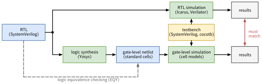
The two checks complement each other. The gate-level simulation only covers the stimuli of the testbench, but it shows what the netlist does from its real, unknown start state. The equivalence check covers every input sequence, but it works with the two values 0 and 1 and starts both designs from the same state, so it cannot see a mismatch that comes from unknown start values (Section 3.3.1). Neither of them tells you how to avoid a mismatch, and debugging a netlist is hard. It consists of thousands of cells with generated names, the FSM states have lost their names, and the hierarchy is flattened. In the final netlist of the counter of the AMS chip template, for example, the outputs of the eight flip-flops are called net3 to net10. It pays to write RTL that cannot cause a mismatch in the first place. Mismatches have only a few root causes:
- Simulation semantics that synthesis ignores: the unknown value
xand initial values. They are the subject of Section 3.3 and Section 3.4.1. - Constructs that tools read differently: incomplete sensitivity lists, the
full_caseandparallel_casepragmas, andunique casewithoutdefault. Section 2 already showed how to avoid them (Section 2.5.5, Section 2.5.13). - Timing that the RTL simulation does not model: glitches of combinational outputs and the delay of a derived clock. Section 3.4.2 and Section 3.5 show how to design them away, and Section 6 covers timing in depth.
3.3 Four-Valued Simulation, Two-Valued Silicon
A variable of type logic has four values (Section 2.5.2): 0, 1, z for high impedance, and x for unknown. Silicon has only two: every node is either low or high, apart from short transitions. An x is the simulator’s way of saying that it does not know which of the two. The most common sources of x are a register without reset before its first load, a net with two conflicting drivers, an explicit assignment of 'x, and an array index out of range.
A perfect simulator would set a signal to x only if it could really be 0 or 1 in the hardware. Such an exact analysis is far too expensive, so the language defines simple rules for every operator and statement instead, and these rules err in both directions:
- X-optimism: the simulation shows a known value where the hardware could have either. An
iftreats an unknown condition as false and takes theelsebranch, and acaseitem never matches an unknown expression, so thedefaultbranch runs. - X-pessimism: the simulation shows
xwhere the hardware has a known value, e.g., because anxthat cancels out in the hardware is still propagated.
The following testbench describes the 2:1 multiplexer of Figure 11 in three ways, plus an AND gate, and sets the select sel to x. The default branch of the case assigns x only for this demonstration.
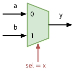
sel = 0 selects a, and sel = 1 selects b. The output y stands for y_if, y_case, and y_cond in the testbench, which sets sel to x. In the hardware, sel is low or high, so y is either a or b.
xprop/testbenches/verilog/xprop_tb.sv
// SPDX-FileCopyrightText: 2026 Simon Dorrer
// SPDX-License-Identifier: Apache-2.0
// Description: Three ways to describe a 2:1 multiplexer, plus an AND
// gate, simulated with an unknown select. Shows how if, case, ?:, and
// & treat x.

`timescale 1ns / 1ps

module xprop_tb;

  logic sel, a, b;
  logic y_if, y_case, y_cond, y_and;

  always_comb begin
    if (sel) y_if = b;
    else     y_if = a;
  end

  always_comb begin
    case (sel)
      1'b0:    y_case = a;
      1'b1:    y_case = b;
      default: y_case = 1'bx;  // only for this demonstration
    endcase
  end

  assign y_cond = sel ? b : a;
  assign y_and  = sel & a;

  initial begin
    sel = 1'bx;
    {a, b} = 2'b01;
    #1 $display("sel=x a=0 b=1: if=%b case=%b ?:=%b and=%b",
                y_if, y_case, y_cond, y_and);
    {a, b} = 2'b11;
    #1 $display("sel=x a=1 b=1: if=%b case=%b ?:=%b and=%b",
                y_if, y_case, y_cond, y_and);
    $finish;
  end

endmodule
Table 22 shows the results in Icarus Verilog and in Verilator, each for two input combinations. For comparison, the fourth row is the gate-level model of the SG13CMOS5L multiplexer cell sg13cmos5l_mux2_1, simulated in Icarus Verilog with the same inputs.
sel = x. Each entry gives the result for a = 0, b = 1 and for a = b = 1.
| Description | Icarus Verilog | Verilator | Hardware |
|---|---|---|---|
if, else |
0 / 1 |
0 / 1 |
0 or 1 / 1 |
case, default assigns x |
x / x |
0 / 1 |
0 or 1 / 1 |
sel ? b : a |
x / 1 |
0 / 1 |
0 or 1 / 1 |
cell sg13cmos5l_mux2_1 |
x / 1 |
not run | 0 or 1 / 1 |
sel & a |
0 / x |
0 / 0 |
0 / 0 or 1 |
Five lessons follow from the table:
ifis optimistic. Witha=0andb=1, it shows a clean0where the hardware could have either value. A bug that leaves a select unknown is invisible behind anif.- A
defaultthat assignsxis pessimistic. Witha=b=1, thecaseshowsx, although the hardware gives1for either select. With a defined default, as in the FSM of Section 3.3.1, thecaseis optimistic like theif. - The conditional operator
?:behaves like the multiplexer cell. For an unknown select, it merges both inputs bit by bit: equal bits stay known, different bits becomex. A multiplexer that synthesis builds from AND and OR gates, however, is pessimistic again, since(x & 1) | (~x & 1)givesx. Even a gate-level simulation is only as exact as its cells. - The AND gate is exact. Icarus Verilog knows that
x & 0is0. - Verilator knows no
x. It is a two-state simulator and replaces everyxby a two-state value, here0, so its results are those ofsel = 0. That makes Verilator fast, but it hides every unknown value. The option--x-assignselects what an explicit'xbecomes, by default the value that simulates fastest. The option--x-initialselects what the variables start with. With its default,unique, they start at0, unless the run-time option+verilator+rand+reset+2asks for random values, and+verilator+seed+<n>selects the seed. Random start values are what silicon does: every flip-flop powers up as0or1, and nobody knows which.
Since an x cannot be trusted in either direction, the guidelines are strict. Never assign 'x in RTL. The lowRISC style guide puts it clearly: “The use of X literals in RTL code is strongly discouraged” (lowRISC 2026). An 'x tells the synthesis tool that it may choose any value, so the netlist can implement a value that the RTL simulation never showed. Assign a defined default instead, as the two-process style does (Section 2.5.7). Do not take the absence of x in an RTL simulation as a proof that a design is defined. Run the regression in Verilator with random start values and several seeds, and simulate the netlist at least once (Section 4). With --x-assign unique, Verilator also randomizes the explicit 'x assignments that slipped through. In testbench checks, compare with !== or $isunknown(), as in Table 21.
3.3.1 The Missing Reset
The most common source of an unknown value is a register without reset. As an example, take the controller FSM of Section 2.5.9 and remove the reset from its state register:
// State register without a reset: its start value is unknown
always_ff @(posedge clk_i) begin
  state_q <= state_d;
end
The complete module is ctrl_fsm_noreset/rtl/ctrl_fsm_noreset.sv. Its testbench prints the first eight clock cycles after power-up, with start_i high in cycle 2 and last_i high in cycle 4. Figure 12 compares four simulations of the same RTL: Icarus Verilog, Verilator with its default start values, Verilator with random start values, and Icarus Verilog with the netlist that Yosys synthesizes onto SG13CMOS5L cells.
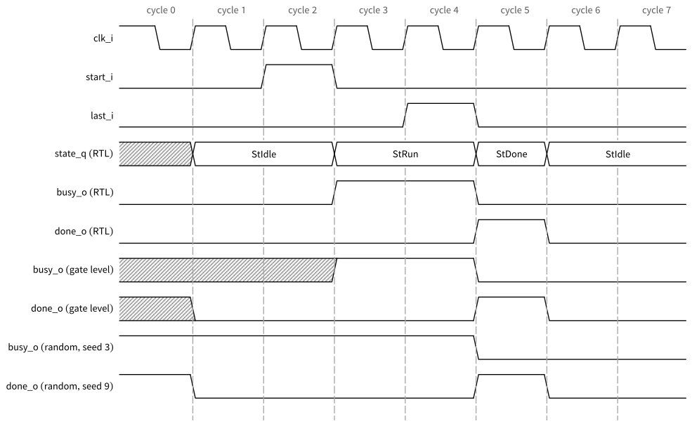
start_i high in cycle 2, last_i in cycle 4). In the RTL simulation, the state starts unknown (hatched), but the default branch returns it to StIdle at the first clock edge, and the outputs never show x. Icarus Verilog and Verilator give the same outputs. The gate-level simulation of the synthesized netlist shows x until start_i forces a known state. With random start values, Verilator shows what the chip can do after power-up: a run that was never started (seed 3) or a done_o pulse for it (seed 9).
- In the RTL simulation with Icarus Verilog,
state_qstarts asxx. Nocaseitem matches, so thedefaultbranch setsstate_dtoStIdle, and the outputs keep their default value0. After the first clock edge, the FSM is inStIdleand works perfectly. The missing reset is invisible: the X-optimism of thecasestatement keeps everyxaway from the outputs. - Verilator starts
state_qat00, which isStIdle. The missing reset is invisible again. - With random start values, Verilator shows what the chip does after power-up. Seed 1 starts in
StIdle(00) and seed 2 in the unused code11, which thedefaultbranch turns intoStIdleafter one cycle. Both are harmless. Seed 3, however, starts inStRun(01):busy_ois high from cycle 0 untillast_iends a run that was never started. Seed 9 starts inStDone(10), anddone_oreports the end of a job that never existed. Which of these a chip shows depends on the die, the supply ramp, and the temperature. - The gate-level simulation of the netlist shows that something is wrong:
busy_oanddone_oarexin cycle 0, andbusy_ostaysxuntilstart_iforces a known state.
The guidelines for resets are therefore:
- Reset every register that holds control state: FSM states, counters, valid flags, and pointers (Section 2.9, rule 8).
- A data register may stay without reset if the control logic guarantees that it is written before it is read, e.g., a pipeline register behind a valid flag, or the content of a memory. Large designs often omit these resets, because the reset net must reach every flip-flop that uses it, and it then needs its own buffer tree and timing checks like a clock. In SG13CMOS5L, a register without reset saves no cell area, though: the library has no flip-flop without reset. Its flip-flops are
dfrbpanddfrbpqand the scan flip-flopssdfrbp,sdfrbpq, andsdfbbp(Section 9), and all of them have a reset input, which synthesis simply ties inactive for a register without reset. - Use the four-state type
logicfor registers, also as the base type of an enumeration. The two-state typesbitandintstart at0in every simulator and hide a missing reset, just like Verilator. In VHDL, a signal of an enumeration type starts with its leftmost value, e.g.,IDLE, so the RTL simulation of a VHDL FSM without reset looks fine as well, while the gate-level simulation showsU.
TipExercise: Find the Missing Reset
Change into the folder content/modeling/code/ctrl_fsm_noreset of the course repository.
Simulate the RTL with Icarus Verilog:
iverilog -g2012 -o rtl.vvp rtl/ctrl_fsm_noreset.sv \
  testbenches/verilog/ctrl_fsm_noreset_tb.sv
vvp rtl.vvp
In which cycle is
state_qunknown? Why do the outputs never show anx?Build the RTL with Verilator once, and run it first with the default start values and then with random ones for ten seeds:
verilator --binary --timing --timescale 1ns/1ps \
  --top-module ctrl_fsm_noreset_tb rtl/ctrl_fsm_noreset.sv \
  testbenches/verilog/ctrl_fsm_noreset_tb.sv
./obj_dir/Vctrl_fsm_noreset_tb
for s in 1 2 3 4 5 6 7 8 9 10; do
  ./obj_dir/Vctrl_fsm_noreset_tb +verilator+rand+reset+2 \
    +verilator+seed+$s | head -1
done
Which start states do the six seeds that the text does not name give? Run seeds 3 and 9 again without
| head -1. How does the controller behave?In
rtl/ctrl_fsm_noreset.sv, change the base type of the enumeration fromlogic [1:0]to the two-statebit [1:0], and repeat step 1. What changes in cycle 0, and why is that dangerous? Restore the file withgit restore rtl/ctrl_fsm_noreset.sv.Synthesize the RTL onto SG13CMOS5L cells and simulate the netlist, with the cell models of the PDK (
$LIBand$CELLSas defined at the beginning of the chapter):yosys -p "read_verilog -sv rtl/ctrl_fsm_noreset.sv; \ synth -top ctrl_fsm_noreset; \ dfflibmap -liberty $LIB; abc -liberty $LIB; opt_clean; \ stat -liberty $LIB; write_verilog -noattr nl.v" iverilog -g2012 -gno-specify -DGL -o gl.vvp \ $CELLS/sg13cmos5l_udp.v $CELLS/sg13cmos5l_stdcell.v nl.v \ testbenches/verilog/ctrl_fsm_noreset_tb.sv vvp gl.vvpWhich flip-flop cells does Yosys use, and how are their reset inputs connected? For the controller with reset, Yosys chooses a one-hot encoding (Section 2.5.9). Does it do so here? In which cycles are
busy_oanddone_ounknown?Which of the simulations reveal the bug, and what does each of them show? How do you fix it?
Before continuing, please finish the previous exercise. Once you are done, compare with the solution below.
TipSolution: Find the Missing Reset
state_qisxxin cycle 0 only:cycle 0: state_q=xx busy_o=0 done_o=0 cycle 1: state_q=00 busy_o=0 done_o=0 cycle 2: state_q=00 busy_o=0 done_o=0 cycle 3: state_q=01 busy_o=1 done_o=0 cycle 4: state_q=01 busy_o=1 done_o=0 cycle 5: state_q=10 busy_o=0 done_o=1 cycle 6: state_q=00 busy_o=0 done_o=0 cycle 7: state_q=00 busy_o=0 done_o=0The outputs are assigned
0by default before thecase, and nocaseitem matchesxx, so they keep their defaults. Thedefaultbranch moves the FSM toStIdleat the first clock edge. Icarus Verilog prints a “sorry” message that it ignores theuniquequalifier (Section 2.5.8), which does not change the result.With the default start values, Verilator prints the same trace, except that
state_qis already00in cycle 0. With random start values, the ten seeds of Verilator 5.052 start in all four codes: seeds 1 and 10 inStIdle(00), seeds 2 and 5 in the unused code11, seeds 3, 4, 6, 7, and 8 inStRun(01), and seed 9 inStDone(10). Another version of Verilator can map the seeds to other start values. From11, thedefaultbranch returns toStIdleafter one cycle. Seed 3 starts inStRun, sobusy_ois high from cycle 0 to cycle 4, untillast_iends a run that was never started. Seed 9 starts inStDone, sodone_ois high in cycle 0. From cycle 5 on, all runs are identical.With
bit [1:0], Icarus Verilog startsstate_qat00, and the trace no longer shows anyx, just like Verilator. A two-state type thus hides a missing reset in every simulator, which is why registers should be of typelogic.Yosys maps the design onto 8 cells, among them two
sg13cmos5l_dfrbpq_1flip-flops. Since the RTL has no reset, theirRESET_Binputs are tied to1'h1. Yosys keeps the binary encoding: its FSM detection reports “Not marking ctrl_fsm_noreset.state_q as FSM state register: Circuit seems to be self-resetting”, because thedefaultbranch returns every unknown state toStIdle, and it leaves such a register alone. In the gate-level simulation,busy_ois unknown in cycles 0 to 2, anddone_oin cycle 0:cycle 0: busy_o=x done_o=x cycle 1: busy_o=x done_o=0 cycle 2: busy_o=x done_o=0 cycle 3: busy_o=1 done_o=0The
defaultbranch does not help here, since in the netlist, gates compute the next state, and they propagate the unknown state. After the first clock edge, the state can only beStIdleorStRun(every other state leads toStIdle), sodone_ois known to be0, whilebusy_ostaysx. In cycle 2,start_imoves both possible states toStRun. The gate-level simulation is exact here: an output isxexactly where the chip can show either value. Icarus Verilog also prints 68 “sorry: ifnone with an edge-sensitive path is not supported” messages for the timing blocks of the cell models, which-gno-specifyskips anyway, and Yosys reports “ABC: Warning: The network is combinational”. Neither affects the result.The RTL simulation in Icarus Verilog, Verilator with its default start values, and a two-state type all hide the bug. The gate-level simulation reveals it: it shows which outputs are undefined after power-up. The random start values show the concrete wrong behaviors, a run and a
done_opulse that nobody started. The fix is the reset of the originalctrl_fsm(Section 2.5.9).
3.4 FPGA Habits That Break on an ASIC
Many of you have designed for FPGAs, and FPGA tools are forgiving. The bitstream initializes every flip-flop of an FPGA based on static RAM (SRAM), the synthesis tool maps arrays and multiplications onto the block RAMs and multipliers of the FPGA, and clock managers and global clock buffers are available as primitives. On an ASIC, every gate comes from the standard-cell library, and the only larger blocks are the macros of the PDK, such as SRAMs and IO cells. Table 23 lists the habits that do not carry over.
| FPGA habit | On an ASIC | Instead |
|---|---|---|
| initial values | dropped by synthesis without a warning | a reset (Section 3.4.1) |
| a register output as clock | a second clock with its own tree | a clock enable (Section 3.4.2) |
| an inferred block RAM | flip-flops, ten times the area | an SRAM macro (Section 3.4.3) |
| an inferred multiplier (DSP block) | a large, slow array of standard cells | a suitable architecture (Section 7) |
| an internal tri-state bus | buffers that can short or float | a multiplexer (Section 3.4.4) |
| clock managers, PLLs, vendor primitives | not in the cell library | analog IP, clock gating (Section 7) |
| the global reset at configuration | no automatic reset | a reset pin and synchronizer (Section 8) |
3.4.1 Initial Values
On an FPGA, a register gets its start value with an initial value in the declaration, and the bitstream loads it at configuration. The LED blinker of the following exercise is written this way:
logic [COUNT_WIDTH-1:0] count_q    = '0;
logic                   slow_clk_q = 1'b0;
logic                   led_q      = 1'b0;
The RTL simulation honors the initial values, and the counter starts at zero in Icarus Verilog and in Verilator. Verilator flags them with -Wall, as step 1 of the following exercise shows. Yosys keeps the initial values through the generic synthesis, but an ASIC flip-flop has no way to implement them, and the mapping onto SG13CMOS5L cells drops them without a single warning in the log. In a gate-level simulation of the blinker with DIV = 4, the counter therefore stays unknown, and led_o is still x after 40 clock cycles, in which it should have toggled five times. On the chip, the registers start with random values. An initial block is for testbenches only (Table 15). In RTL, the reset sets the start values.
3.4.2 Clock Dividers and Clock Enables
On an FPGA, it is sometimes common (but not recommended) to divide a clock with a register and to clock another register with its output, as in Figure 13 (a). On an ASIC, such a divided clock causes several problems:
- A second clock. All registers clocked by
slow_clk_qrun on a clock of their own. It is derived fromclk_i, so the paths between the two clocks are synchronous and can be timed, but each of them must be timed with the delay between the two clock edges. - A second clock tree. Clock tree synthesis (Section 10) builds a balanced tree for every clock. The divided clock arrives later than
clk_iby the clock-to-output delay of the divider and the delay of its own tree, so the two clocks are skewed, which leads to hold violations on the paths between them unless the trees are balanced against each other. - Constraints. Static timing analysis only knows the clocks it is told about. A register output used as a clock needs a generated clock in the constraints (Section 6), otherwise the paths it clocks are not analyzed at all.
- Test. The scan test must control every clock in the design (Section 9).
- Simulation. Without a reset or an initial value, the divider starts as
xand never produces an edge, so the registers behind it never change.
The solution is a clock enable, Figure 13 (b). Every rising edge of the divided clock becomes a pulse tick that is high for one cycle of clk_i, like the strobe of the tick generator in Section 2.5.7. The register stays on clk_i and only loads a new value while tick is high, otherwise it keeps its value (Section 2.5.6). The design keeps one clock, one clock tree, and one set of constraints. Where a block really needs a lower clock frequency, its clock comes from a dedicated clock generation block and is declared in the constraints. To save power, the clock of an idle block is switched off with a clock gating cell instead (Section 7). Neither of them is a register output that happens to toggle somewhere in the logic.
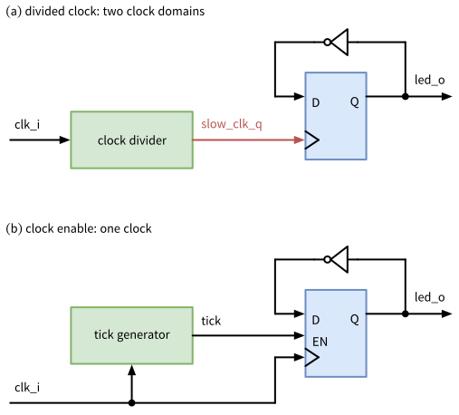
slow_clk_q clocks the register: the design now has two clocks, and slow_clk_q needs its own clock tree and constraints. (b) Every rising edge of the old divided clock becomes a one-cycle pulse tick, which enables the register. All registers stay on clk_i.
Figure 14 compares the two circuits over time. In (a), the register sees every clock edge one clock-to-output delay late, so led_o changes after two of these delays. In (b), tick is an ordinary synchronous signal: it changes shortly after a rising edge of clk_i, and the next rising edge samples it like any other register input. led_o then changes after one clock-to-output delay.
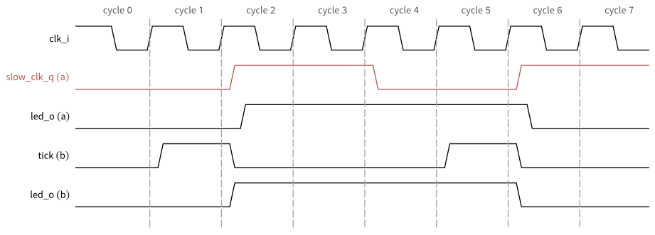
DIV = 2. A register output does not change exactly at the clock edge, but one clock-to-output delay after it. The figure exaggerates this delay and leaves out the delay of a clock tree. led_o toggles in the same cycles in both circuits. (a) slow_clk_q lags clk_i by one clock-to-output delay, and led_o by two, because slow_clk_q clocks its register. (b) tick comes from registers on clk_i, so it lags clk_i as well. It is high in the cycle before the clock edge at which led_o toggles, and it falls only after this edge, so the edge still samples it high. led_o lags clk_i by one clock-to-output delay.
TipExercise: An LED Blinker from FPGA to ASIC
The file content/modeling/code/led_blink/exercise/led_blink_fpga.sv is an LED blinker written with FPGA habits:
led_blink/exercise/led_blink_fpga.sv
// SPDX-FileCopyrightText: 2026 Simon Dorrer
// SPDX-License-Identifier: Apache-2.0
// Description: LED blinker written with FPGA habits. With a 50 MHz
// clock and the default DIV, slow_clk_q runs at 2 Hz and led_o blinks
// at 1 Hz. Works on an FPGA, but is not ready for an ASIC.

`default_nettype none

module led_blink_fpga #(
  parameter int unsigned DIV = 12_500_000
) (
  input  logic clk_i,
  output logic led_o
);

  localparam int unsigned      COUNT_WIDTH = $clog2(DIV);
  localparam [COUNT_WIDTH-1:0] COUNT_LAST  = COUNT_WIDTH'(DIV - 1);

  logic [COUNT_WIDTH-1:0] count_q    = '0;
  logic                   slow_clk_q = 1'b0;
  logic                   led_q      = 1'b0;

  // Clock divider: slow_clk_q toggles every DIV clock cycles
  always_ff @(posedge clk_i) begin
    if (count_q == COUNT_LAST) begin
      count_q    <= '0;
      slow_clk_q <= ~slow_clk_q;
    end else begin
      count_q <= count_q + 1'b1;
    end
  end

  // The LED toggles at every rising edge of the divided clock
  always_ff @(posedge slow_clk_q) begin
    led_q <= ~led_q;
  end

  assign led_o = led_q;

endmodule

`default_nettype wire
Change into the folder content/modeling/code/led_blink. Its rtl/ already holds the solution, so move it out of the way first with mv rtl/led_blink.sv led_blink_solution.sv, and compare at the end.
- Lint the file with
verilator --lint-only -Wall exercise/led_blink_fpga.svand explain the warnings. - List all FPGA habits in the file, and explain what happens to each of them on an ASIC.
- Draw the block diagram of an ASIC version
led_blinkwith only one clock,clk_i, and an asynchronous active-low resetrst_ni. Which registers do you need, and which of them need an enable? - Implement
led_blinkinrtl/led_blink.svin the two-process style, with the parameterDIVand the portsclk_i,rst_ni, andled_o. After the reset,led_omust toggle every2*DIVclock cycles, exactly as in the FPGA version. Lint your file. - Run the cocotb testbench on both versions, in the folder
testbenches/cocotb:TOPLEVEL=led_blink_fpga python3 led_blink_tb.pyandpython3 led_blink_tb.py. Run your version also withSIM=verilator. - Synthesize both versions with
yosys -p "read_verilog -sv <file>; synth -top <module>; stat"and compare the flip-flop types. Which clock does each flip-flop use?
Before continuing, please finish the previous exercise. Once you are done, compare with the solution below.
TipSolution: An LED Blinker from FPGA to ASIC
- Verilator reports
PROCASSINITthree times, once for each ofcount_q,slow_clk_q, andled_q: the registers have initial values instead of a reset. - The file has three FPGA habits. The initial values are dropped by the ASIC synthesis, so all registers start with random values, and the gate-level simulation stays
x(Section 3.4.1).slow_clk_qis a register output used as a clock, which creates a second clock with its own clock tree and constraints (Section 3.4.2). And the design has no reset, so neither the simulation nor the chip has a defined start. - The block diagram is Figure 13 (b), with the tick generator made of two registers. All three registers run on
clk_i: the countercount_q, the registerphase_q, which takes over the role ofslow_clk_q, andled_q.count_qwraps everyDIVcycles (wrap).phase_qtoggles at everywrap, so the old divided clock would rise exactly whenwrapcomes whilephase_qis low. This is the enabletickofled_q.phase_qalso needs an enable (wrap),count_qdoes not. - The ASIC version follows below.
phase_qis in fact one more bit of the counter: a counter that wraps every2*DIVcycles would do the same job, withtickat its wrap-around.
led_blink/rtl/led_blink.sv
// SPDX-FileCopyrightText: 2026 Simon Dorrer
// SPDX-License-Identifier: Apache-2.0
// Description: LED blinker for an ASIC, with the same timing as
// led_blink_fpga: led_o toggles every 2*DIV clock cycles. A clock
// enable (tick) replaces the divided clock, and a reset replaces the
// initial values.

`default_nettype none

module led_blink #(
  parameter int unsigned DIV = 12_500_000
) (
  input  logic clk_i,
  input  logic rst_ni,
  output logic led_o
);

  localparam int unsigned      COUNT_WIDTH = $clog2(DIV);
  localparam [COUNT_WIDTH-1:0] COUNT_LAST  = COUNT_WIDTH'(DIV - 1);

  logic [COUNT_WIDTH-1:0] count_d, count_q;
  logic                   phase_d, phase_q;  // was slow_clk_q
  logic                   led_d, led_q;
  logic                   wrap, tick;

  // Register process: one clock, one reset for all registers
  always_ff @(posedge clk_i or negedge rst_ni) begin
    if (!rst_ni) begin
      count_q <= '0;
      phase_q <= 1'b0;
      led_q   <= 1'b0;
    end else begin
      count_q <= count_d;
      phase_q <= phase_d;
      led_q   <= led_d;
    end
  end

  // wrap: every DIV clock cycles. tick: where slow_clk_q of the FPGA
  // version would rise, a one-cycle enable instead of a clock edge
  assign wrap = (count_q == COUNT_LAST);
  assign tick = wrap & ~phase_q;

  // Combinational process: defaults first, then all decisions
  always_comb begin
    count_d = count_q + 1'b1;
    phase_d = phase_q;
    led_d   = led_q;
    if (wrap) begin
      count_d = '0;
      phase_d = ~phase_q;
    end
    if (tick) begin
      led_d = ~led_q;
    end
  end

  assign led_o = led_q;

endmodule

`default_nettype wire
- All runs end with
TESTS=1 PASS=1 FAIL=0 SKIP=0. In the RTL simulation, both versions behave identically: the testbench checks thatled_otoggles exactly every2*DIVcycles, withDIV = 4. - In the FPGA version, Yosys 0.70 builds 108 generic cells with 26 flip-flops: 24
$_SDFF_PP0_for the counter (it has recognized the wrap-around to zero as a synchronous reset), one$_DFFE_PP_forslow_clk_qwith the wrap-around as enable, and one$_DFF_P_forled_q, which runs onposedge slow_clk_q. In the ASIC version, all 26 flip-flops run onclk_iwith the resetrst_ni: 24$_DFF_PN0_for the counter and two$_DFFE_PN0P_forphase_qandled_q, with their enables. The ASIC version needs 117 generic cells, a few more than the FPGA version, because the asynchronous reset keeps Yosys from merging the wrap-around to zero into the flip-flops as a synchronous reset. Withoutrst_ni, the same RTL needs 110 cells.
3.4.3 Memories: Flip-Flops or SRAM Macros
On an FPGA, an array with a synchronous write and read, as in the following listing, infers the block RAM of Figure 15:
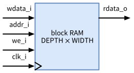
DEPTH words of WIDTH bits. At a rising edge of clk_i, it stores wdata_i at the address addr_i if we_i is high, and it reads the word at addr_i to rdata_o, so the read data appear one clock cycle after the address.
ram_ff/rtl/ram_ff.sv
// SPDX-FileCopyrightText: 2026 Simon Dorrer
// SPDX-License-Identifier: Apache-2.0
// Description: Single-port memory with synchronous write and read,
// written as an array. On an FPGA, this infers a block RAM. On an
// ASIC, Yosys builds it from flip-flops and multiplexers.

`default_nettype none

module ram_ff #(
  parameter int unsigned DEPTH = 256,
  parameter int unsigned WIDTH = 8
) (
  input  logic                     clk_i,
  input  logic                     we_i,
  input  logic [$clog2(DEPTH)-1:0] addr_i,
  input  logic [WIDTH-1:0]         wdata_i,
  output logic [WIDTH-1:0]         rdata_o
);

  logic [WIDTH-1:0] mem_q [DEPTH];
  logic [WIDTH-1:0] rdata_q;

  // No reset: the content of a memory is undefined after power-up
  always_ff @(posedge clk_i) begin
    if (we_i) begin
      mem_q[addr_i] <= wdata_i;
    end
    rdata_q <= mem_q[addr_i];
  end

  assign rdata_o = rdata_q;

endmodule

`default_nettype wire
On an ASIC, Yosys builds the same RTL from standard cells: a flip-flop for every bit, a multiplexer in front of each flip-flop that keeps its value while the word is not written (the library has no flip-flop with an enable input), and a tree of multiplexers for the read port. Figure 16 shows this structure for a very small memory of two words of one bit.
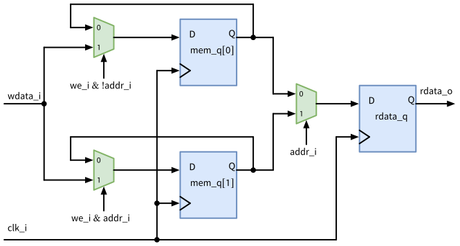
ram_ff with DEPTH = 2 and WIDTH = 1 after synthesis with Yosys: three sg13cmos5l_dfrbpq_1 flip-flops, three sg13cmos5l_mux2_1 multiplexers, and two gates for the write decoder, whose functions label the selects of mem_q[0] and mem_q[1]. Input 0 of such a multiplexer feeds the output of the flip-flop back, so the bit keeps its value. Input 1 loads wdata_i while this word is written. The read multiplexer selects the word at addr_i, and rdata_q holds it for the next clock cycle. ABC maps the multiplexer of mem_q[1] with swapped inputs and an inverted select, which is the same function.
For 256 words of 8 bits, Yosys needs 2056 sg13cmos5l_dfrbpq_1 flip-flops (2048 for the content and 8 for the read data), 2074 sg13cmos5l_mux2_1 cells, most of them the multiplexers that keep the values, and 368 sg13cmos5l_mux4_1 cells, most of them the read tree. In total, that is 165,743 µm² of cell area, or 81 µm² per bit. The SG13CMOS5L PDK, however, also provides SRAM macros ($PDK_ROOT/ihp-sg13cmos5l/libs.ref/sg13cmos5l_sram). The single-port macro RM_IHPSG13_1P_256x8_c3_bm_bist stores the same 256 words of 8 bits in 236.8 µm × 74.1 µm = 17,547 µm², 8.6 µm² per bit, which is about 9.4 times less, even before the routing of the flip-flop version is counted. Even a memory of 32 words of 8 bits needs 20,944 µm² of flip-flops and multiplexers, more than the smallest SRAM macro of the PDK, RM_IHPSG13_1P_64x16_c2 with 1024 bits in 236.8 µm × 64.36 µm = 15,240 µm².
Use flip-flops for small memories, e.g., a first-in first-out buffer (FIFO) of a few words, and for memories with several read ports, such as the register file of a CPU with two read ports and one write port. The PDK has single-port macros (RM_IHPSG13_1P_*) and two-port macros (RM_IHPSG13_2P_*), but none with more ports. For everything larger, use an SRAM macro. It is a hard macro, like the macros of the AMS chip template: the RTL instantiates it by name, and the PDK provides its simulation model, its timing library, its abstract in the Library Exchange Format (LEF) for place and route, and its layout. Its read data appear one clock cycle after the address, as in ram_ff, but details such as the behavior when a read and a write hit the same address can differ, so check them in the simulation model before you replace an array. The macros with _bm_bist in their names also offer a bit mask for the write data and a second set of ports for a memory test, which a test controller in the design drives (Section 9).
3.4.4 Tri-States
On a circuit board, several chips share a bus through tri-state drivers. Inside an FPGA, the tools convert such a bus into multiplexers. Inside an ASIC, a tri-state bus is a real tri-state bus, as Figure 17 and the following listing show:
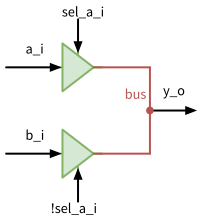
z) and leaves the net bus to the other driver.
pitfalls/bus_tri.sv
// SPDX-FileCopyrightText: 2026 Simon Dorrer
// SPDX-License-Identifier: Apache-2.0
// Description: An internal tri-state bus with two drivers, an FPGA
// and board-level habit. Do not use this on chip, write a
// multiplexer.

`default_nettype none

module bus_tri (
  input  logic       sel_a_i,
  input  logic [7:0] a_i,
  input  logic [7:0] b_i,
  output logic [7:0] y_o
);

  tri [7:0] bus;

  assign bus = sel_a_i  ? a_i : 8'bz;  // driver A
  assign bus = !sel_a_i ? b_i : 8'bz;  // driver B
  assign y_o = bus;

endmodule

`default_nettype wire
Verilator lints this file without a warning. A plain synth in Yosys 0.70 warns that “Yosys has only limited support for tri-state logic at the moment” and then stops with an error, because the output y_o is “already driven” by the other driver. LibreLane runs the extra pass tribuf and maps the drivers onto the tri-state buffers sg13cmos5l_ebufn_2 of the library, so it would build the bus. Do not use one anyway. If two enables overlap, two drivers fight, and a large current flows. If no enable is active, the bus floats, the gates that read it draw cross current, and the simulation shows x. Tri-states also complicate the timing analysis and the scan test. The lowRISC style guide forbids them: “Do not use three-state logic (Z state) to accomplish on-chip logic such as muxing” (lowRISC 2026). Write a multiplexer, here assign y_o = sel_a_i ? a_i : b_i;. Tri-states belong to the bidirectional pads of the padframe (Section 10).
3.5 Macro Boundaries
A chip built with the AMS chip template consists of macros that are hardened separately and then assembled into the chip top level (Section 1.10). Two properties of a macro boundary decide how easy this assembly is: whether the timing of a macro depends on its neighbors, and whether the macro can be verified at gate level with its RTL testbench.
3.5.1 Registered Inputs and Outputs
When LibreLane hardens a macro, it does not know the logic outside. It assumes that the environment uses a fixed part of the clock period on each side: the constraints of the template set the input and output delays to IO_DELAY_CONSTRAINT, by default 20 % of the clock period, i.e., 4 ns of the 20 ns period of the counter macro. A path from an input to a register of the macro may then use the remaining 80 %, and a combinational path from an input to an output only 60 %, both a little less after the setup time and the clock uncertainty. If the logic outside is slower than assumed, the chip fails timing, although every macro met its own constraints. Figure 18 (a) shows such a path through two macros.
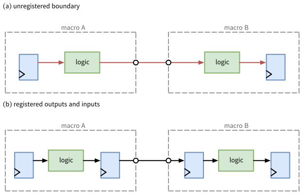
With registered outputs, every output of a macro comes directly from a flip-flop, Figure 18 (b). The paths through the logic of a macro end at this register, and the next macro sees a stable signal right after the clock edge, so the timing of each macro depends only on its own logic. What remains between the macros is a wire from register to register, which has almost a full clock cycle and is easy to time at the top level. Outputs from flip-flops are also free of glitches, which matters when they drive a pad, another clock domain, or an asynchronous input. Register the inputs as well when they come from another macro far away on the die, so that the long wire gets a full clock cycle. Asynchronous inputs from pads need a synchronizer anyway (Section 8). The price is a clock cycle of latency for every register stage.
3.5.2 Ports That Survive Synthesis
The template simulates a macro with the same cocotb testbench at RTL and at gate level, the latter with make sim-gl-cocotb (Table 20). This only works if the testbench sees the same interface in both cases:
- Plain
logicvectors at the top-level ports. Inside the macro, structures, enumerations, and arrays are fine, but after synthesis, every port is a plain vector of bits, and a testbench that relies on a structure or an interface at the top level cannot drive the netlist. - No top-level parameters that the testbench changes. The netlist is synthesized for one set of parameter values, and the gate-level testbench must use exactly these values. A testbench that sets a parameter, such as
DIV = 4inled_blink_tb.py, needs a netlist synthesized with that value. - Access only the ports. Internal names do not reliably survive synthesis and place and route. In the synthesized netlist of the template counter, the outputs of the flip-flops are still called
counter_value_o, but in its final netlist, they arenet3tonet10(Section 3.2). A testbench that reads an internal signal works at RTL and fails at gate level. - A reset at the start of every test, and no reliance on initial values, since the netlist starts as
x.
3.6 Architecture Determines the Result
Logic synthesis optimizes the logic you describe, but it does not invent a new architecture. A binary counter stays a binary counter, and a shift register stays a shift register. An adder written with + becomes a fast adder only if the synthesis tool knows a fast architecture for it (Section 7). The choice of the architecture is yours, and it decides area and speed much more than the details of the code.
3.6.1 Case Study: The Exclusive Counter
An exclusive counter has eight outputs q_o[7:0], of which exactly one is high at any time (a one-hot code). Its specification:
- After the asynchronous active-low reset
rst_ni,q_o[0]is high. - The synchronous clear
clr_imakesq_o[0]high at the next rising clock edge. It has priority overen_i. - While
en_iis high, the high bit moves up by one position at every rising clock edge and wraps around fromq_o[7]toq_o[0]. Whileen_iis low,q_okeeps its value.
For example, a 3-bit one-hot counter cycles through this repeating sequence: 001, 010, 100 and then loops back to 001. A valid one-hot counter never displays 000 or multiple 1 simultaneously during normal operation.
Figure 19 shows two architectures for this function. The first one counts in binary with three flip-flops and decodes the count into the one-hot code:
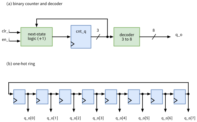
cnt_q and a decoder: few flip-flops, but the outputs come from combinational logic. (b) A one-hot ring of eight flip-flops: each output comes directly from a flip-flop. All flip-flops run on clk_i with the reset rst_ni (not drawn for simplicity). In (b), the multiplexers in front of the D inputs that implement clr_i and en_i are not drawn.
excl_cnt/rtl/excl_cnt_bin.sv
// SPDX-FileCopyrightText: 2026 Simon Dorrer
// SPDX-License-Identifier: Apache-2.0
// Description: Exclusive counter, architecture 1: a 3-bit binary
// counter and a decoder. Exactly one of the eight bits of q_o is
// high. clr_i (synchronous, priority over en_i) and the reset select
// q_o[0], en_i moves the high bit up by one and wraps from q_o[7] to
// q_o[0].

`default_nettype none

module excl_cnt_bin (
  input  logic       clk_i,
  input  logic       rst_ni,
  input  logic       clr_i,
  input  logic       en_i,
  output logic [7:0] q_o
);

  logic [2:0] cnt_d, cnt_q;

  // Register process
  always_ff @(posedge clk_i or negedge rst_ni) begin
    if (!rst_ni) begin
      cnt_q <= '0;
    end else begin
      cnt_q <= cnt_d;
    end
  end

  // Combinational process: the 3-bit counter wraps by itself
  always_comb begin
    cnt_d = cnt_q;
    if (clr_i) begin
      cnt_d = '0;
    end else if (en_i) begin
      cnt_d = cnt_q + 3'd1;
    end
  end

  // Decoder: the outputs come from combinational logic
  assign q_o = 8'b0000_0001 << cnt_q;

endmodule

`default_nettype wire
The second one stores the one-hot code directly in a ring of eight flip-flops and rotates it:
excl_cnt/rtl/excl_cnt_ring.sv
// SPDX-FileCopyrightText: 2026 Simon Dorrer
// SPDX-License-Identifier: Apache-2.0
// Description: Exclusive counter, architecture 2: a one-hot ring of
// eight flip-flops, same behavior as excl_cnt_bin. clr_i
// (synchronous, priority over en_i) and the reset select q_o[0], en_i
// rotates the high bit up by one and wraps from q_o[7] to q_o[0].

`default_nettype none

module excl_cnt_ring (
  input  logic       clk_i,
  input  logic       rst_ni,
  input  logic       clr_i,
  input  logic       en_i,
  output logic [7:0] q_o
);

  logic [7:0] q_d, q_q;

  // Register process: the reset value is the first one-hot code
  always_ff @(posedge clk_i or negedge rst_ni) begin
    if (!rst_ni) begin
      q_q <= 8'b0000_0001;
    end else begin
      q_q <= q_d;
    end
  end

  // Combinational process: rotate left by one bit
  always_comb begin
    q_d = q_q;
    if (clr_i) begin
      q_d = 8'b0000_0001;
    end else if (en_i) begin
      q_d = {q_q[6:0], q_q[7]};
    end
  end

  // The outputs come directly from the flip-flops
  assign q_o = q_q;

endmodule

`default_nettype wire
The cocotb testbench excl_cnt/testbenches/cocotb/excl_cnt_tb.py checks the reset value, a full count with wrap-around, and 500 cycles of random clr_i and en_i against a model, and both architectures pass. To compare them, each one is synthesized onto SG13CMOS5L cells with the Yosys command of the exercise in Section 3.3.1, and the netlist is analyzed with the static timing analyzer OpenSTA, using the script excl_cnt/syn/sta.tcl. It assumes a 100 MHz clock without a clock tree, inputs that change at the clock edge, and a load of 10 fF at every output. Section 6 explains these timing constraints. Table 24 lists the results.
| Binary counter and decoder | One-hot ring | |
|---|---|---|
| flip-flops | 3 | 8 |
| standard cells | 22 | 28 |
| cell area | 308.4 µm² | 553.2 µm² |
| longest path from the clock to an output | 0.49 ns | 0.23 ns |
| longest path between two flip-flops | 0.52 ns | 0.31 ns |
- The ring needs 79 % more area. Flip-flops are expensive: a
sg13cmos5l_dfrbpq_1has 49.0 µm², a 3-input NOR gatesg13cmos5l_nor3_1only 9.1 µm². The eight flip-flops of the ring take 392 of its 553 µm². - The ring is faster. Its outputs come directly from the flip-flops, so the path from the clock to an output is just the clock-to-output delay of 0.23 ns. In the binary version, the decoder adds two gates, and the incrementer in front of the flip-flops makes the path between them longer as well.
- The ring has clean outputs. Outputs from flip-flops are free of glitches. The decoder outputs of the binary version can glitch when several counter bits change at once, e.g., from
011to100. This matters whenq_oleaves the macro, drives a pad, or selects something in another clock domain (Section 3.5). - The binary version is more robust. Its outputs are one-hot by construction, whatever the counter holds. The ring is one-hot only as long as its state is: if it starts without a reset, or if a bit flips, e.g., from radiation, the ring can hold no high bit or several of them until the next
clr_i. For the ring, the reset is mandatory.
Neither architecture is better in general: the requirements decide. Note what did not matter here: the coding style. The file excl_cnt/rtl/excl_cnt_ring_for.sv describes the ring with a for loop instead of the concatenation, and writes the clear last, so that it overrides the rotation instead of being checked first. Yosys synthesizes it into exactly the same 28 cells with 553.2 µm². What synthesis sees is the function of every register, not the syntax that describes it.
TipExercise: A Third Architecture, the Johnson Counter
A Johnson counter (twisted ring counter) of four flip-flops s_q[3:0] shifts left and feeds the inverted most significant bit back into the least significant bit: s_d = {s_q[2:0], ~s_q[3]}. As an exclusive counter, the reset and clr_i load 0000, and the k-th state of the sequence (counted from 0) drives q_o[k]. Change into the folder content/modeling/code of the course repository. The folder excl_cnt/rtl already holds the solution, so move it out of the way first with mv excl_cnt/rtl/excl_cnt_johnson.sv excl_cnt_johnson_solution.sv.
Draw the Johnson counter with its four flip-flops, in the style of Figure 19 (b): the connections between the flip-flops, the inverted feedback, and a decoder block that generates
q_o. As in that figure, leave out the clock and reset wires and the multiplexers forclr_ianden_i.Starting from
0000, write down the sequence of its states. After how many steps does it repeat?In the sequence, every state differs from the next one in exactly one bit. Show that two neighboring bits of the ring identify every state (
s_q[3]ands_q[0]count as neighbors too), and write down the decoder for the eight outputs with one 2-input AND gate each (inputs may be inverted).Implement
excl_cnt_johnsoninexcl_cnt/rtl/excl_cnt_johnson.svwith the same ports and behavior as the other two architectures. Lint it and run the testbench inexcl_cnt/testbenches/cocotbwithTOPLEVEL=excl_cnt_johnson python3 excl_cnt_tb.py.Synthesize your design onto SG13CMOS5L cells and analyze its timing, both in the folder
excl_cnt:yosys -p "read_verilog -sv rtl/excl_cnt_johnson.sv; \ synth -top excl_cnt_johnson; \ dfflibmap -liberty $LIB; abc -liberty $LIB; opt_clean; \ stat -liberty $LIB; write_verilog -noattr excl_cnt_johnson.nl.v" TOP=excl_cnt_johnson sta -no_init -exit syn/sta.tclAdd a column to Table 24.
Rank the three architectures by area and by speed. Which one would you choose (a) for the smallest area, (b) for outputs that go to another clock domain, where a glitch can be captured as a pulse, and (c) for the highest clock frequency?
Before continuing, please finish the previous exercise. Once you are done, compare with the solution below.
TipSolution: A Third Architecture, the Johnson Counter
- Figure 20 shows the counter. It is the ring of Figure 19 (b) with four flip-flops and an inverter in the feedback, plus a decoder as in Figure 19 (a), here from 4 to 8 bits.
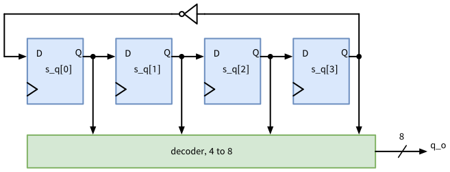
s_q[0] to s_q[3], and the inverted s_q[3] returns to s_q[0]. All four outputs drive the decoder. All flip-flops run on clk_i with the reset rst_ni (not drawn for simplicity), and the multiplexers in front of the D inputs that implement clr_i and en_i are not drawn, as in Figure 19 (b).
- The sequence is
0000,0001,0011,0111,1111,1110,1100,1000, and then0000again: four flip-flops pass through eight states. - Within the sequence, the ones fill up from the right and then the zeros. A state is therefore identified by the position of its single 0-1 or 1-0 edge between two neighboring bits, or, for
0000and1111, by the equal bitss_q[3]ands_q[0]at both ends. Each output is one 2-input AND gate, as in the decoder of the following listing.
excl_cnt/rtl/excl_cnt_johnson.sv
// SPDX-FileCopyrightText: 2026 Simon Dorrer
// SPDX-License-Identifier: Apache-2.0
// Description: Exclusive counter, architecture 3: a 4-bit Johnson
// counter (twisted ring) and a decoder of 2-input gates, same
// behavior as excl_cnt_bin. The Johnson counter passes through the
// eight states 0000, 0001, 0011, 0111, 1111, 1110, 1100, 1000.

`default_nettype none

module excl_cnt_johnson (
  input  logic       clk_i,
  input  logic       rst_ni,
  input  logic       clr_i,
  input  logic       en_i,
  output logic [7:0] q_o
);

  logic [3:0] s_d, s_q;

  // Register process
  always_ff @(posedge clk_i or negedge rst_ni) begin
    if (!rst_ni) begin
      s_q <= '0;
    end else begin
      s_q <= s_d;
    end
  end

  // Combinational process: shift left, feed back the inverted MSB
  always_comb begin
    s_d = s_q;
    if (clr_i) begin
      s_d = '0;
    end else if (en_i) begin
      s_d = {s_q[2:0], ~s_q[3]};
    end
  end

  // Decoder: every state differs from its neighbors in one bit, so
  // two adjacent bits identify it
  assign q_o[0] = ~s_q[3] & ~s_q[0];  // 0000
  assign q_o[1] =  s_q[0] & ~s_q[1];  // 0001
  assign q_o[2] =  s_q[1] & ~s_q[2];  // 0011
  assign q_o[3] =  s_q[2] & ~s_q[3];  // 0111
  assign q_o[4] =  s_q[3] &  s_q[0];  // 1111
  assign q_o[5] =  s_q[1] & ~s_q[0];  // 1110
  assign q_o[6] =  s_q[2] & ~s_q[1];  // 1100
  assign q_o[7] =  s_q[3] & ~s_q[2];  // 1000

endmodule

`default_nettype wire
- Lint and all three tests pass (
TESTS=3 PASS=3 FAIL=0 SKIP=0). - The Johnson counter needs 4 flip-flops and 24 cells with 368.3 µm². Its longest path from the clock to an output and its longest path between two flip-flops are both 0.35 ns.
- By area, the binary version is the smallest (308.4 µm²), followed by the Johnson counter (368.3 µm²) and the ring (553.2 µm²). By speed, the ring is the fastest (0.23 ns from the clock to an output), followed by the Johnson counter (0.35 ns) and the binary version (0.49 ns). (a) The binary version is the smallest, and its outputs are one-hot by construction. (b) Only the ring has outputs that come directly from flip-flops and never glitch. The Johnson counter comes close: while it counts, only one bit of its state changes per step, and each output depends on only two bits, so a decoder of 2-input gates cannot glitch, unlike the binary decoder, where up to three bits change at once. A clear from, e.g.,
0111to0000, however, changes three bits at once, and then the Johnson decoder can glitch as well. (c) For the highest clock frequency, the ring is the best choice. Like the ring, the Johnson counter needs its reset: its eight unused states form a second cycle of their own, e.g.,0010,0101,1011, in which several outputs are high, and the counter never leaves it withoutclr_i.
3.7 Checklist for Synthesizable, ASIC-Ready RTL
The coding guidelines of Section 2.9 make your RTL correct and readable. The following checklist adds the guidelines of this chapter, which make it ready for an ASIC:
- Every register that holds control state has a reset. Data registers may stay without reset if they are written before they are read.
- No initial values and no
initialblocks in RTL. - No
'xassignments. Every variable gets a defined default value. - One clock per macro if possible. No clock comes from a register or from logic: a clock enable replaces a divided clock.
- Memories with more than a few hundred bits are SRAM macros. Flip-flop arrays are for small memories and for memories with several read ports.
- No internal tri-states. Tri-states only exist in the pads.
- Every output of a macro comes from a flip-flop. Inputs from far away get a register, asynchronous inputs from pads a synchronizer.
- The top-level ports are plain
logicvectors, and the testbench accesses only the ports. - The architecture comes first. Compare the candidates with a quick synthesis and timing analysis before you optimize the code.
- Simulate with more than one tool: Icarus Verilog with four values, Verilator with random start values, and the netlist at gate level.
3.8 Summary
- You verify the RTL, but the chip implements the netlist. Their simulations must agree, and the guidelines of this chapter remove the most common causes of a mismatch.
- Simulators approximate the unknown value
x:ifand acasewith a defined default are optimistic and hide an unknown select or state, a default that assignsxis pessimistic, the conditional operator matches the multiplexer cell, and Verilator replaces everyxby a two-state value. Never assign'xin RTL, and do not trust an RTL simulation withoutx. - A missing reset hides in the RTL simulation. Random start values in Verilator and the gate-level simulation reveal it. Reset all control state. In SG13CMOS5L, every flip-flop has a reset input anyway.
- FPGA habits do not carry over: initial values are dropped by synthesis without a warning, a divided clock creates a second clock with its own tree, an inferred memory is built from flip-flops with about ten times the area of an SRAM macro, and an internal tri-state bus either fails to synthesize or risks shorts and floating nodes.
- Replace a divided clock by a clock enable: every rising edge of the slow clock becomes a one-cycle pulse that enables registers on the main clock.
- Register the outputs of every macro, so that its timing does not depend on its neighbors, and keep the top-level ports plain, so that the same testbench runs on the netlist.
- The architecture decides area and speed. For the exclusive counter, the binary version is the smallest, the one-hot ring the fastest, and the Johnson counter lies in between. Two codings of the same architecture gave the same netlist.
In Section 4, we take the testbenches of the last two chapters to a systematic verification methodology, including the gate-level simulation of a netlist with the same testbench.
4 Functional Verification with cocotb
The last two chapters used testbenches: a few lines of SystemVerilog or Python that drive a design and check its outputs. This chapter turns them into a methodology. Three questions guide it. How does a testbench decide that a design is correct, without anybody looking at waveforms? Which stimuli does it apply, if it cannot apply all of them? And when is the verification complete? The answers are a testbench architecture with a reference model, a mix of directed, exhaustive, and random stimuli, and the measurement of coverage. Along the way, we check the checks themselves with deliberate bugs, and we run the same testbench on the synthesized netlist, without and with the delays of the cells.
Note
All code of this chapter is available in the folder content/verification/code of the course repository, with one folder per design. As in Section 3, the RTL is in rtl/, the cocotb testbenches are in testbenches/cocotb/, and the files of an exercise are in exercise/. The assertions of the FIFO are in testbenches/sva/, its testbench for the comparison of the simulators is in testbenches/verilog/, and its timing analysis script is in syn/. Every file in rtl/ lints without warnings and synthesizes. All numbers in this chapter come from the IIC-OSIC-TOOLS image 2026.10 (Verilator 5.052, Icarus Verilog 14.0, cocotb 2.1.0, Yosys 0.70, OpenSTA 3.1.0) and the typical-corner library of SG13CMOS5L (sg13cmos5l_stdcell_typ_1p20V_25C.lib, 1.2 V, 25 °C). Run times depend on the computer, and the ones quoted here come from a laptop. The script scripts/check_verification.sh reproduces all other numbers: run bash scripts/check_verification.sh in the container from the root of the repository.
For the exercises, clone the course repository into your designs folder once, if you have not done so yet:
cd /foss/designs
git clone https://github.com/iic-jku/vlsi-design.git
The gate-level part of this chapter synthesizes a design onto the standard cells of SG13CMOS5L. Define the path of the cell library in every new terminal:
LIB=$PDK_ROOT/ihp-sg13cmos5l/libs.ref/sg13cmos5l_stdcell/lib
LIB=$LIB/sg13cmos5l_stdcell_typ_1p20V_25C.lib
4.1 Learning Objectives
After this chapter, you will be able to:
- distinguish verification, test, and validation, and name what each verification method can prove
- write a verification plan that gives each feature of a specification a check and a coverage goal
- structure a cocotb testbench into generator, driver, monitor, reference model, scoreboard, and coverage
- choose between directed, exhaustive, and constrained-random stimuli, estimate the run time of an exhaustive test, and reproduce a random test from its seed
- measure code coverage with Verilator and functional coverage in Python, and explain why full coverage does not prove a correct design
- write SystemVerilog assertions in a separate checker, attach them with
bind, and know which open-source tools support them - judge the quality of a testbench with mutation testing
- run the same testbench on the synthesized netlist, without and with the cell delays of an SDF file, and explain why a timing simulation does not replace static timing analysis
- explain how Icarus Verilog and Verilator work, and choose between them for a task
- set up a regression that fails when a test fails
4.2 Why Verification Matters
A chip cannot be patched. A bug in software is fixed with an update, but a bug in the masks of an ASIC is in every die of the wafer. The fix takes a new tapeout: new masks, a new run through the fab, new packaging, and new tests, which costs months and, in advanced technologies, millions of euros. The cost of a bug grows with every step of the flow that it passes. At RTL, a fix takes minutes and a new simulation. After synthesis or layout, it takes another run of the flow. On silicon, it takes a new tapeout. This is why verification takes a large share of the effort in every ASIC project, often more than writing the RTL.
Three terms are easily confused:
- Verification asks whether the design does what its specification says. It works on models of the chip, i.e., the RTL, the netlist, and the layout, and it happens before the tapeout. This chapter covers functional verification, which checks the logic behavior of the design, cycle by cycle.
- Test asks whether a manufactured die is free of defects. It runs on every die after fabrication, with test patterns that the design for test of Section 9 prepares. A test assumes that the design itself is correct.
- Validation asks whether the chip does what its application needs, e.g., on a board with real signals and software. It happens with the first silicon.
Verification has several methods, and each one answers a different question (Table 25).
| Method | Question it answers | Limit | In this course |
|---|---|---|---|
| Simulation | Does the design behave correctly for the applied stimuli? | covers only the stimuli you apply | this chapter |
| Logic equivalence checking | Does the netlist implement the same function as the RTL? | no timing, and the RTL itself must be correct | Section 5 |
| Static timing analysis | Does every path meet its timing constraint? | only as good as the constraints, no function | Section 6 |
| Formal property checking | Does a property hold for every possible input sequence? | limited to small blocks | outlook only |
| FPGA prototyping and emulation | Does the design run its real software? | needs a working design and extra hardware | outlook only |
Simulation remains the workhorse. It works for every design and at every level, from the RTL to the netlist with delays. Its fundamental limit is just as clear: a simulation can show that a bug exists, but never that no bug is left. Everything in this chapter aims at making the simulated stimuli count: checking every output automatically, steering the stimuli into the corners of the design, and measuring what they have reached.
4.3 A Synchronous FIFO as Running Example
A first-in, first-out memory (FIFO) buffers data between a producer and a consumer that do not always run at the same rate. It makes a good example for verification: its interface is simple, but its behavior depends on the history of all pushes and pops, and the bugs hide in its corner cases, i.e., a full or an empty FIFO, a push and a pop in the same cycle, and the wrap-around of the pointers. Its asynchronous version, which connects two clock domains, follows in Section 8. Figure 21 shows our FIFO as a block, with the producer on the left and the consumer on the right.
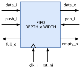
DEPTH entries of WIDTH bits. The producer writes on the left, and full_o tells it that the FIFO refuses a push. The consumer reads on the right, and empty_o tells it that data_o holds no entry. clk_i clocks the FIFO, and rst_ni empties it.
The specification of our FIFO:
- The FIFO stores up to
DEPTH = 4entries ofWIDTH = 8bits. - With
push_ihigh, the FIFO storesdata_iat the next rising clock edge, but only if it is not full. Withpop_ihigh, it removes the oldest entry, but only if it is not empty. - A push and a pop in the same cycle are allowed, and each one follows its own rule. On a full FIFO, the pop removes an entry and the push is refused. On an empty FIFO, the push stores an entry and the pop is refused.
data_oshows the oldest entry whileempty_ois low (first-word fall-through). While the FIFO is empty,data_ois undefined.full_oandempty_oshow the state after the last clock edge. After the reset, the FIFO is empty.
The third rule is a design decision. Many FIFOs accept a push on a full FIFO if a pop happens in the same cycle. Ours refuses it, and the specification must say so, because the testbench checks the specification, not the RTL. The RTL follows the two-process style of Section 2.5.7:
fifo/rtl/fifo.sv
// SPDX-FileCopyrightText: 2026 Simon Dorrer
// SPDX-License-Identifier: Apache-2.0
// Description: Synchronous FIFO with first-word fall-through: data_o
// shows the oldest entry while empty_o is low. A push is accepted
// only while the FIFO is not full, a pop only while it is not empty.

`default_nettype none

module fifo #(
  parameter int unsigned WIDTH = 8,
  parameter int unsigned DEPTH = 4  // power of two, at least 2
) (
  input  logic             clk_i,
  input  logic             rst_ni,
  input  logic             push_i,
  input  logic [WIDTH-1:0] data_i,
  input  logic             pop_i,
  output logic [WIDTH-1:0] data_o,
  output logic             full_o,
  output logic             empty_o
);

  localparam int unsigned AW = $clog2(DEPTH);

  // One bit more than the address: the extra wrap bit tells a full
  // FIFO (same address, different wrap bit) from an empty one
  logic [AW:0]      wr_ptr_d, wr_ptr_q, rd_ptr_d, rd_ptr_q;
  logic [WIDTH-1:0] mem_q [DEPTH];
  logic             push, pop;

  // Register process
  always_ff @(posedge clk_i or negedge rst_ni) begin
    if (!rst_ni) begin
      wr_ptr_q <= '0;
      rd_ptr_q <= '0;
    end else begin
      wr_ptr_q <= wr_ptr_d;
      rd_ptr_q <= rd_ptr_d;
    end
  end

  // Storage without reset: a pop never reads an unwritten entry
  always_ff @(posedge clk_i) begin
    if (push) begin
      mem_q[wr_ptr_q[AW-1:0]] <= data_i;
    end
  end

  // Combinational process
  always_comb begin
    push     = push_i && !full_o;
    pop      = pop_i && !empty_o;
    wr_ptr_d = push ? wr_ptr_q + 1'b1 : wr_ptr_q;
    rd_ptr_d = pop ? rd_ptr_q + 1'b1 : rd_ptr_q;
  end

  // Status flags and read port, decoded from the registers only
  assign empty_o = (wr_ptr_q == rd_ptr_q);
  assign full_o  = (wr_ptr_q == {~rd_ptr_q[AW], rd_ptr_q[AW-1:0]});
  assign data_o  = mem_q[rd_ptr_q[AW-1:0]];

endmodule

`default_nettype wire
The storage mem_q holds four entries, organized as a ring (Figure 22). The write pointer addresses the next free entry, and the read pointer the oldest one. Each pointer has one bit more than the address, the wrap bit, which toggles each time the pointer wraps around. The difference of the two pointers, taken modulo 8, is therefore the number of entries, from 0 to 4. With the address bits alone, a full and an empty FIFO would look the same, because both pointers address the same entry. The flags therefore compare the whole pointers: equal pointers mean empty, and equal addresses with different wrap bits mean full.
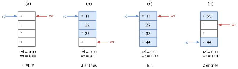
DEPTH = 4: four entries, which the pointers use as a ring, addressed by the two lower bits of the pointers. The write pointer wr points at the next free entry and the read pointer rd at the oldest entry, which data_o shows. Both pointers have a third bit, the wrap bit, which toggles each time a pointer wraps from entry 3 to entry 0. Below each panel, a pointer is written as wrap bit and address, e.g., 1 00. (a) After the reset, both pointers are equal: empty. (b) After three pushes. (c) After four pushes, both pointers address entry 0 again, and only the different wrap bits tell full from empty. (d) After three pops and one more push, the two entries wrap around the end of the storage.
Figure 23 shows the hardware that the RTL describes. As in Section 3.4.3, the storage has no reset. A pop never reads an entry that was not written, so its start value does not matter, and only the pointers are reset. The flags and data_o are decoded from the registers only, without a path from an input to an output.
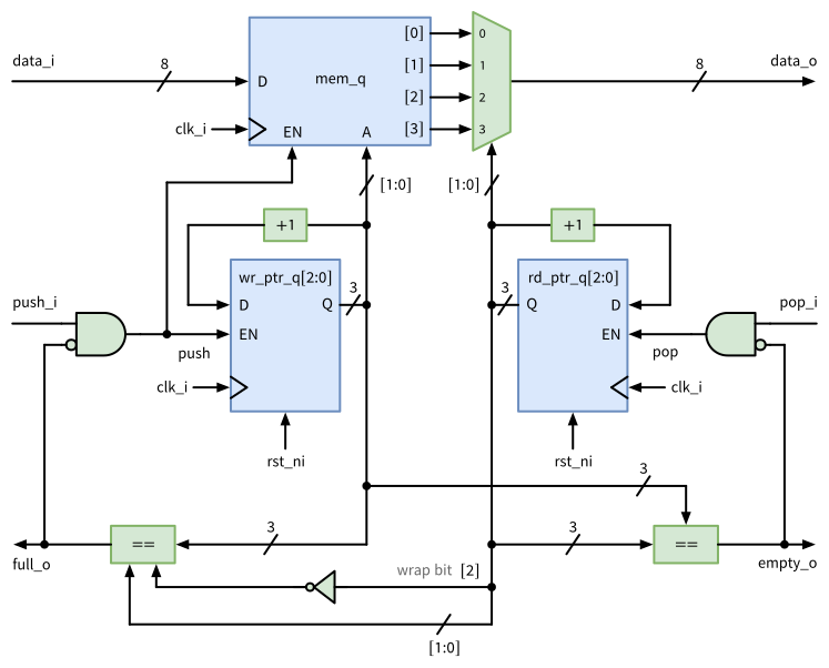
fifo.sv with DEPTH = 4 and WIDTH = 8, with the registers in blue and the combinational logic in green. A slash marks a bus with its width or with the bits that a branch takes. The storage mem_q has no reset. While push is high, a rising edge of clk_i stores data_i in the entry at the address A, the bits wr_ptr_q[1:0]. The read multiplexer shows the entry at rd_ptr_q[1:0] at data_o, without a clock edge. Each pointer is a 3-bit register with the reset rst_ni and loads its value plus 1 while its enable EN is high. The RTL keeps a pointer with a multiplexer, which the figure draws as this enable, as Yosys maps it. The two comparators decode the flags from the whole pointers only: empty_o compares both 3-bit pointers, and full_o compares wr_ptr_q with {~rd_ptr_q[2], rd_ptr_q[1:0]}, the read pointer with its wrap bit inverted. The two AND gates refuse a push into a full FIFO and a pop from an empty one.
4.4 The Verification Plan
Before writing a testbench, write down what has to be verified. A verification plan lists the features of the specification and gives each one a check, i.e., how the testbench notices a failure, and a coverage goal, i.e., how you know that the stimulus has exercised the feature. The verification is complete when every check passes and every coverage goal is reached, not when the testbench runs without errors. A testbench without checks also runs without errors. Table 26 shows the plan for the FIFO, and the rest of this chapter builds the testbench, the assertions, and the coverage measurement that it asks for.
| Feature of the specification | Check | Coverage goal |
|---|---|---|
| Entries come out in the order they went in | the scoreboard compares data_o with a model in every cycle |
pushes and pops in every fill state |
empty_o after the reset and when drained, full_o with four entries |
the scoreboard compares both flags in every cycle | the FIFO was empty, partially filled, and full |
| A full FIFO refuses a push | scoreboard, assertions a_room and a_level |
a push, and a push with a pop, on a full FIFO |
| An empty FIFO refuses a pop | scoreboard, assertion a_level |
a pop, and a pop with a push, on an empty FIFO |
| The oldest entry stays until it is popped | scoreboard, assertion a_head |
cycles without a pop on a partially filled and on a full FIFO |
| The netlist behaves like the RTL | gate-level simulation with the same testbench | all of the above |
4.5 Anatomy of a Testbench
The testbenches of Section 2.6 drive the inputs and check the outputs in one loop. That works for a small block, but it mixes three concerns: which operations to apply, how to apply them at the pins, and what the correct answer is. Larger testbenches separate them into the blocks of Figure 24. They work with transactions, i.e., operations at a higher level than single pin values, e.g., “push the value 0x11”:
- The generator creates the transactions, as a directed list or at random (Section 4.6).
- The driver turns each transaction into pin values at the inputs of the design under test (DUT), at the right time.
- The monitor observes the pins at the inputs and outputs of the DUT and turns them back into transactions. It never drives a signal.
- The reference model computes what the DUT must do. It is written from the specification, not from the RTL, and it is much simpler than the RTL, because it does not have to be synthesizable.
- The scoreboard compares what the DUT did with what the model expects, and reports every difference.
- The coverage collector counts which situations the stimulus has reached (Section 4.7).
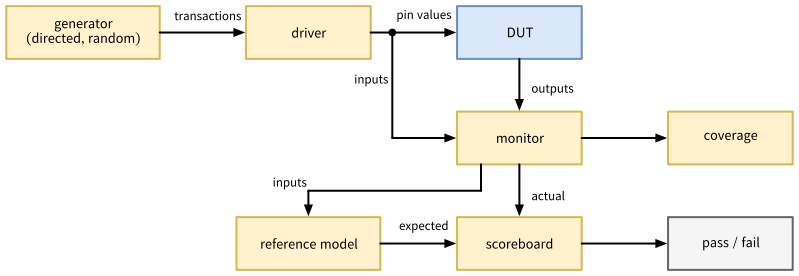
In industry, testbenches with this structure are written in SystemVerilog with the Universal Verification Methodology (UVM) (IEEE 2020), a class library with a standard set of base classes for all these blocks. cocotb builds the same structure from plain Python, and the IIC-OSIC-TOOLS image also contains pyuvm (pyuvm developers 2026), an implementation of UVM in Python on top of cocotb. For the FIFO, a few functions and one class are enough:
fifo/testbenches/cocotb/fifo_tb.py
# SPDX-FileCopyrightText: 2026 Simon Dorrer
# SPDX-License-Identifier: Apache-2.0
# Description: cocotb testbench for the FIFO with a driver, a monitor,
# a reference model, a scoreboard, and functional coverage.
# Environment variables: SIM=verilator builds with code coverage, and
# SVA=1 adds the assertions of testbenches/sva. GL=1 (Icarus only)
# simulates the netlist fifo.nl.v of the macro folder, SDF=1 adds the
# delays of fifo.sdf. CLK_PERIOD_NS sets the clock (default 20), and
# CHECK=0 switches the scoreboard checks off.

import os
import random
from collections import Counter, deque
from pathlib import Path

import cocotb
from cocotb.clock import Clock
from cocotb.triggers import ClockCycles, FallingEdge, ReadOnly
from cocotb_tools.runner import get_results, get_runner

DEPTH = 4
WIDTH = 8
CLK_PERIOD_NS = float(os.getenv("CLK_PERIOD_NS", "20"))
CHECK = os.getenv("CHECK", "1") == "1"


class Scoreboard:
    """Reference model of the specification, checks, and coverage."""

    def __init__(self):
        self.model = deque()  # oldest entry first
        self.coverage = Counter()

    def check(self, full, empty, data):
        """Compare the outputs of the DUT with the model."""
        n = len(self.model)
        assert full == (n == DEPTH), f"full_o = {full}, {n} entries"
        assert empty == (n == 0), f"empty_o = {empty}, {n} entries"
        if n > 0:
            assert data == self.model[0], \
                f"data_o = {data}, expected {self.model[0]:0{WIDTH}b}"

    def update(self, push, data, pop):
        """Count coverage, then apply one clock edge to the model."""
        full, empty = len(self.model) == DEPTH, len(self.model) == 0
        state = "full" if full else "empty" if empty else "partial"
        op = ["idle", "pop", "push", "push+pop"][2 * push + pop]
        self.coverage[f"{op} when {state}"] += 1
        if pop and not empty:
            self.model.popleft()
        if push and not full:  # a full FIFO refuses a push
            self.model.append(data)


async def monitor(dut, sb):
    """Sample the DUT at every falling edge, after the driver."""
    while True:
        await ReadOnly()
        if CHECK:
            sb.check(dut.full_o.value, dut.empty_o.value,
                     dut.data_o.value)
        sb.update(int(dut.push_i.value), int(dut.data_i.value),
                  int(dut.pop_i.value))
        await FallingEdge(dut.clk_i)


async def driver(dut, transactions):
    """Apply one (push, data, pop) transaction per clock cycle."""
    for push, data, pop in transactions:
        dut.push_i.value = push
        dut.data_i.value = data
        dut.pop_i.value = pop
        await FallingEdge(dut.clk_i)
    dut.push_i.value = 0
    dut.pop_i.value = 0
    await ClockCycles(dut.clk_i, 2)


async def start_up(dut):
    """Start the clock, reset the DUT, and start the monitor."""
    cocotb.start_soon(Clock(dut.clk_i, CLK_PERIOD_NS, "ns").start())
    dut.rst_ni.value = 0
    dut.push_i.value = 0
    dut.data_i.value = 0
    dut.pop_i.value = 0
    await ClockCycles(dut.clk_i, 2)
    await FallingEdge(dut.clk_i)
    dut.rst_ni.value = 1
    sb = Scoreboard()
    cocotb.start_soon(monitor(dut, sb))
    return sb


def report(sb):
    """Log the coverage bins, return the bins that were never hit."""
    bins = [f"{op} when {state}"
            for op in ("idle", "push", "pop", "push+pop")
            for state in ("empty", "partial", "full")]
    for name in bins:
        cocotb.log.info(f"{name:24s} {sb.coverage[name]:5d}")
    return [name for name in bins if sb.coverage[name] == 0]


@cocotb.test()
async def test_fill_and_drain(dut):
    """Directed: push DEPTH values, then pop all of them."""
    sb = await start_up(dut)
    values = [0x11 * (i + 1) for i in range(DEPTH)]
    await driver(dut, [(1, v, 0) for v in values]
                 + [(0, 0, 1)] * DEPTH)
    report(sb)


@cocotb.test()
async def test_random(dut):
    """Random: phases of 50 cycles that tend to fill or to drain."""
    sb = await start_up(dut)
    transactions = []
    for _ in range(20):
        p_push = random.choice([0.2, 0.5, 0.8])
        for _ in range(50):
            push = int(random.random() < p_push)
            pop = int(random.random() < 1 - p_push)
            data = random.getrandbits(WIDTH)
            transactions.append((push, data, pop))
    await driver(dut, transactions)
    holes = report(sb)
    assert not holes, f"coverage holes: {holes}"


def fifo_runner():
    sim = os.getenv("SIM", "icarus")
    proj_path = Path(__file__).resolve().parent
    macro_path = proj_path / "../.."

    top = "fifo"
    sources = [macro_path / "rtl/fifo.sv"]
    sva = macro_path / "testbenches/sva/fifo_sva.sv"
    build_args, plusargs = [], []
    if sim == "verilator":
        build_args = ["--coverage"]
        if os.getenv("SVA", "0") == "1":
            sources.append(sva)
    if os.getenv("GL", "0") == "1":
        cells = Path(os.environ["PDK_ROOT"]) \
            / "ihp-sg13cmos5l/libs.ref/sg13cmos5l_stdcell/verilog"
        sources = [cells / "sg13cmos5l_udp.v",
                   cells / "sg13cmos5l_stdcell.v",
                   macro_path / "fifo.nl.v"]
        build_args = ["-gno-specify"]
        if os.getenv("SDF", "0") == "1":
            top = "fifo_sdf"
            sources.append(proj_path / "fifo_sdf.sv")
            build_args = ["-gspecify"]
            sdf_file = (macro_path / "fifo.sdf").resolve()
            plusargs = [f"+SDF={sdf_file}"]

    runner = get_runner(sim)
    runner.build(
        sources=sources,
        hdl_toplevel=top,
        build_args=build_args,
        always=True,
        waves=True,
        timescale=("1ns", "1ps"),
    )
    results_xml = runner.test(
        hdl_toplevel=top,
        test_module="fifo_tb",
        plusargs=plusargs,
        waves=True,
    )

    # A failing test leaves the exit status at 0, so check the results
    num_tests, num_failed = get_results(results_xml)
    if num_failed:
        raise SystemExit(
            f"FAIL: {num_failed} of {num_tests} tests failed")


if __name__ == "__main__":
    fifo_runner()
- In this small testbench, the class
Scoreboardholds three blocks of Figure 24: the reference model (modelandupdate()), the scoreboard itself (check()), and the coverage collector (coverage, printed byreport()). The generator is the list of transactions in each test. - The reference model is a Python
dequewith the oldest entry first. Compare it with the RTL: no pointers, no wrap bit, and no storage array. This independence is the point. A model that copied the structure of the RTL would also copy its bugs. check()compares both flags in every cycle anddata_owhenever the model holds an entry. It does not checkdata_owhile the FIFO is empty, because the specification leaves it undefined.update()first counts the coverage and then applies one clock edge to the model, with the flags from before the edge, exactly as the specification says.driver()applies one transaction per clock cycle, right after the falling edge, as in Section 2.6.monitor()runs in parallel with the test, started withcocotb.start_soon(). At every falling edge, it waits forReadOnly(), the phase at the end of a time step in which all signals have settled and no process may write anymore. At that moment, the outputs show the state after the last rising edge, and the inputs show what the driver has just applied for the next one. So the monitor first checks the outputs against the model, and then updates the model with the inputs. WithoutReadOnly(), the monitor would still see the inputs from before the writes of the driver, because cocotb applies writes later in the time step.- A failing
assertin the monitor fails the test that is running, with the message of the assertion. test_fill_and_drainis a directed test andtest_randoma random one (Section 4.6). Both print the coverage at the end.- The runner reads the environment variables listed at the top of the file. They select the simulator, the assertions, and the netlist with or without delays, which the following sections use.
Run the testbench in its folder:
cd /foss/designs/vlsi-design/content/verification/code/fifo
cd testbenches/cocotb
COCOTB_RANDOM_SEED=1 python3 fifo_tb.py
cd ../..
Both tests pass, and each one prints a table of its coverage bins, which Section 4.7 explains. COCOTB_RANDOM_SEED fixes the random numbers (Section 4.6.3).
4.6 Stimulus
A testbench is only as good as its stimulus: a bug that the stimulus never activates cannot be found by any check. There are three basic kinds of stimuli, and good testbenches combine them.
4.6.1 Directed Tests
A directed test applies a sequence that a person has written for one feature. test_fill_and_drain pushes four values and pops them again. Directed tests are easy to read and to debug, and they are the right tool for a known corner case, e.g., the reset or the largest value of a counter. Their weakness: they test exactly what their author thought of, and the author of a testbench tends to think of the same cases as the author of the RTL, who is often the same person.
4.6.2 Exhaustive Tests
The ideal stimulus applies every possible input. For a combinational block with \(n\) input bits, these are \(2^n\) input vectors, and an exhaustive test proves the function, at least in simulation. The number grows quickly. A 16-bit multiplier has \(2^{32} \approx 4.3 \cdot 10^{9}\) combinations of its two operands, and a 32-bit adder \(2^{64} \approx 1.8 \cdot 10^{19}\). At 100,000 vectors per second, a good rate for a cocotb testbench, the exhaustive test of the multiplier takes about half a day, and that of the adder almost six million years.
For sequential circuits, it is worse, because the outputs depend on the sequence of all previous inputs. The FIFO has 10 input bits (push_i, pop_i, and data_i), so there are \(2^{10} = 1024\) possible inputs in every cycle and \(1024^{10} \approx 1.3 \cdot 10^{30}\) different sequences of only ten cycles. Exhaustive simulation is therefore limited to small combinational blocks, and to small parameter values of a parameterized design.
4.6.3 Random Tests
A random test applies a large number of random inputs. It finds bugs in cases that nobody thought of, at a low cost per test. The random numbers come from a pseudo-random number generator, whose sequence is fully determined by its start value, the seed. cocotb seeds the random module of Python at the start of every run, from the time or from the environment variable COCOTB_RANDOM_SEED, and prints the seed at the start of the simulation, e.g., Seeding Python random module with 1793394914. When a random test fails, rerun it with this seed to reproduce the failure exactly:
COCOTB_RANDOM_SEED=1793394914 python3 fifo_tb.pyThis works only as long as the testbench draws its random numbers in the same order, so fix the bug before you change the testbench. All results of this chapter use seed 1.
Purely random inputs are not always good stimuli. The interesting states of a design are often reached only by a particular sequence, e.g., a deep FIFO is full only after many more pushes than pops. test_random therefore uses constrained-random stimuli. It runs 20 phases of 50 cycles, i.e., 1000 cycles, and each phase draws the probability of a push from 0.2, 0.5, and 0.8 and sets the probability of a pop to the complement. A phase with mostly pushes fills the FIFO, and a phase with mostly pops drains it. The constraints steer the stimuli toward the corners, and the random values within them still reach combinations that nobody has written down. SystemVerilog has a whole constraint language for this (rand, constraint, and randomize()), and in Python, plain code does the job.
The best tests combine directed and random values: directed values at the corners of every input, i.e., the smallest and the largest value, single bits, and the boundaries of every range, followed by random values. The following exercise shows why.
TipExercise: Verify a Barrel Shifter
The folder barrel_shift contains a combinational barrel shifter in rtl/barrel_shift.sv. It has the parameter WIDTH (a power of two, default 8), the inputs data_i (WIDTH bits), shamt_i ($clog2(WIDTH) bits), and mode_i (2 bits), and the output data_o. mode_i selects a shift left (00), a shift right (01), a rotation left (10), or a rotation right (11) of data_i by shamt_i positions, and a shift fills the free positions with zeros. The folder testbenches/cocotb holds the reference solution, so move it out of the way first. All commands start in the folder barrel_shift:
cd /foss/designs/vlsi-design/content/verification/code/barrel_shift
mv testbenches/cocotb/barrel_shift_tb.py barrel_shift_tb_solution.py- Draw the testbench for the barrel shifter in the style of Figure 24. Which blocks does a combinational DUT need, and which ones merge?
- Write a cocotb testbench
testbenches/cocotb/barrel_shift_tb.pywith a reference model in Python and a testtest_exhaustive, which applies all input vectors of the 8-bit version. Let the runner readWIDTHfrom an environment variable (default 8) and pass it to the DUT as a parameter, and skip the exhaustive test forWIDTHabove 8 with the decorator@cocotb.test(skip=WIDTH > 8). Run the testbench with Icarus Verilog and with Verilator, and note the run time of the test, which cocotb prints in its summary. - Estimate from your measurement how long the exhaustive test would take for
WIDTH = 16and forWIDTH = 32. - Add a test
test_random. It first applies corner values (zero, all ones, only the lowest bit, only the highest bit, and alternating bits, each with the shift amounts 0, 1, andWIDTH - 1and all four modes) and then 10,000 random vectors. Run it withWIDTH=32. - The file
exercise/barrel_shift_bug.svcontains the modulebarrel_shift_bug, with the same ports and one bug. Let your runner select it with the environment variableTOPLEVEL=barrel_shift_bug, as the testbenches of Section 3 do, and run both tests withWIDTH8 and 32. Which test finds the bug, and why does the other one miss it? Then lint the file, once without and once with-GWIDTH=32.
The commands of steps 2, 4, and 5:
cd testbenches/cocotb
python3 barrel_shift_tb.py                 # Icarus Verilog
SIM=verilator python3 barrel_shift_tb.py   # Verilator
WIDTH=32 python3 barrel_shift_tb.py
TOPLEVEL=barrel_shift_bug python3 barrel_shift_tb.py
TOPLEVEL=barrel_shift_bug WIDTH=32 python3 barrel_shift_tb.py
cd ../..
verilator --lint-only -Wall exercise/barrel_shift_bug.sv
verilator --lint-only -Wall -GWIDTH=32 exercise/barrel_shift_bug.sv
Before continuing, please finish the previous exercise. Once you are done, compare with the solution below.
TipSolution: Verify a Barrel Shifter
- The generator creates the input vectors, in nested loops or at random. Since the DUT has no clock and no state, the driver and the monitor merge into one function: apply a vector, wait for the logic to settle, and read the output. The reference model computes the expected output from the same vector, and an
assertcompares them as the scoreboard. In the listing below,check()does all of this in one short function. - The reference testbench:
barrel_shift/testbenches/cocotb/barrel_shift_tb.py
# SPDX-FileCopyrightText: 2026 Simon Dorrer
# SPDX-License-Identifier: Apache-2.0
# Description: Self-checking cocotb testbench for barrel_shift with a
# Python reference model, an exhaustive test (WIDTH <= 8 only), and a
# random test with corner values. WIDTH (default 8) sets the DUT
# parameter, TOPLEVEL=barrel_shift_bug selects the exercise version.

import os
import random
import time
from pathlib import Path

import cocotb
from cocotb.triggers import Timer
from cocotb_tools.runner import get_results, get_runner

WIDTH = int(os.getenv("WIDTH", "8"))
MASK = (1 << WIDTH) - 1
NUM_RANDOM = 10_000


def model(data, shamt, mode):
    """Reference model: what barrel_shift must compute."""
    if mode == 0:
        return (data << shamt) & MASK
    if mode == 1:
        return data >> shamt
    if mode == 2:
        return ((data << shamt) | (data >> (WIDTH - shamt))) & MASK
    return ((data >> shamt) | (data << (WIDTH - shamt))) & MASK


async def check(dut, data, shamt, mode):
    """Apply one input vector and compare data_o with the model."""
    dut.data_i.value = data
    dut.shamt_i.value = shamt
    dut.mode_i.value = mode
    await Timer(1, "ns")
    expected = model(data, shamt, mode)
    assert dut.data_o.value == expected, (
        f"data {data:#x}, shamt {shamt}, mode {mode}: "
        f"expected {expected:0{WIDTH}b}, got {dut.data_o.value}")


@cocotb.test(skip=WIDTH > 8)
async def test_exhaustive(dut):
    """All 2**WIDTH * WIDTH * 4 input vectors."""
    start = time.perf_counter()
    for data in range(1 << WIDTH):
        for shamt in range(WIDTH):
            for mode in range(4):
                await check(dut, data, shamt, mode)
    num = (1 << WIDTH) * WIDTH * 4
    rate = num / (time.perf_counter() - start)
    cocotb.log.info(f"{num} vectors, {rate:.0f} vectors/s")


@cocotb.test()
async def test_random(dut):
    """Corner values first, then NUM_RANDOM random vectors."""
    corners = [0, MASK, 1, 1 << (WIDTH - 1), 0x5555_5555 & MASK]
    for data in corners:
        for shamt in (0, 1, WIDTH - 1):
            for mode in range(4):
                await check(dut, data, shamt, mode)
    for _ in range(NUM_RANDOM):
        await check(dut, random.getrandbits(WIDTH),
                    random.randrange(WIDTH), random.randrange(4))


def barrel_shift_runner():
    sim = os.getenv("SIM", "icarus")
    top = os.getenv("TOPLEVEL", "barrel_shift")
    proj_path = Path(__file__).resolve().parent
    folder = "exercise" if top == "barrel_shift_bug" else "rtl"

    runner = get_runner(sim)
    runner.build(
        sources=[proj_path / f"../../{folder}/{top}.sv"],
        hdl_toplevel=top,
        parameters={"WIDTH": WIDTH},
        always=True,
        timescale=("1ns", "1ps"),
    )
    results_xml = runner.test(
        hdl_toplevel=top,
        test_module="barrel_shift_tb",
    )

    # A failing test leaves the exit status at 0, so check the results
    num_tests, num_failed = get_results(results_xml)
    if num_failed:
        raise SystemExit(
            f"FAIL: {num_failed} of {num_tests} tests failed")


if __name__ == "__main__":
    barrel_shift_runner()
The model uses the unlimited integers of Python and masks the result to WIDTH bits. For a rotation by 0, it shifts by WIDTH in the other direction, which gives 0, as in the RTL. check() applies a vector, waits 1 ns, and compares. The exhaustive test of the 8-bit version applies \(2^8 \cdot 8 \cdot 4 = 8192\) vectors in about 0.1 s, i.e., about 70,000 vectors per second with Icarus Verilog and 100,000 with Verilator. For such a small DUT, the Python side of cocotb limits the rate, so Verilator is only about 1.4 times faster.
- The 16-bit version has \(2^{16} \cdot 16 \cdot 4\) = 4,194,304 vectors, which takes about one minute (measured with the skip limit raised to 16: 64 s with Icarus Verilog and 47 s with Verilator). The 32-bit version has \(2^{32} \cdot 32 \cdot 4 \approx 5.5 \cdot 10^{11}\) vectors, which would take two to three months at these rates.
test_randompasses forWIDTH=32.- With
WIDTH8, both tests pass. WithWIDTH32,test_randomfails at the first corner vector with the shift amount 31 and nonzero data:data 0xffffffff, shamt 31, mode 0gives11111111111111111111111110000000instead of a 1 followed by 31 zeros. The data was shifted by 7 instead of 31 positions. The bug is the declarationlogic [2:0] sh: three bits are enough forWIDTH = 8, but forWIDTH = 32the assignment cutsshamt_idown to its three lower bits. The exhaustive test is a complete proof for the 8-bit instance, but it says nothing about the 32-bit one. Verilator lint is clean with the default parameter, and it reportsWIDTHTRUNC(andUNUSEDSIGNALforshamt_i[4:3]) only with-GWIDTH=32. Verilator even refuses to build the 32-bit version for cocotb:SIM=verilatorstops at the warningWIDTHTRUNC, which it treats as an error, before any test runs. Lint and simulate every parameter value that you use. An exhaustive test at a small parameter value complements a random test at the real one, but does not replace it.
4.7 Coverage
Coverage answers the question of when the verification is complete. It measures what the stimuli have reached. Two kinds complement each other: code coverage, which the simulator measures on the RTL, and functional coverage, which the testbench measures on the specification.
4.7.1 Code Coverage
Code coverage needs no work in the testbench. The simulator counts how often each part of the RTL was exercised. Verilator distinguishes:
- line coverage: was every block of statements executed?
- branch coverage: did every
if,case, and conditional operator take each of its branches? - expression coverage: did the terms of every logical expression, e.g.,
push_iandfull_oinpush_i && !full_o, take the values that decide its result? - toggle coverage: did every bit of every signal change from 0 to 1 and from 1 to 0?
The runner of fifo_tb.py builds with --coverage when you select Verilator, and the simulation writes the counts into sim_build/coverage.dat. The tool verilator_coverage summarizes them and writes a copy of the RTL with the counts in front of every line. The environment variable COCOTB_TEST_FILTER selects the tests to run by name, here only the directed one:
cd /foss/designs/vlsi-design/content/verification/code/fifo
cd testbenches/cocotb
SIM=verilator COCOTB_TEST_FILTER=test_fill_and_drain \
  python3 fifo_tb.py
verilator_coverage --annotate-min 1 --annotate-points \
  --annotate annotated sim_build/coverage.dat
Coverage Summary: (excerpt)
line : 100.0% ( 3/ 3)
toggle : 50.7% ( 69/136)
branch : 100.0% ( 8/ 8)
expr : 100.0% ( 14/ 14)The directed test reaches 100 % line, branch, and expression coverage. The full expression coverage is surprising, since the test never pushes into a full FIFO. But Verilator counts a term as covered when it alone decides the result: the point (full_o==1) => 0 of push_i && !full_o is hit whenever the FIFO is full, with or without a push. Only the toggle coverage shows a gap. The annotated copy annotated/fifo.sv marks every partially covered line by ~ and, thanks to --annotate-points, lists the points below it, e.g.:
~000002   logic [AW:0]      wr_ptr_d, wr_ptr_q, rd_ptr_d, rd_ptr_q;
-000000  point: type=toggle comment=wr_ptr_q[2]:1->0 hier=fifo
The wrap bits of both pointers rise once but never fall, because four pushes and four pops wrap each pointer only once. Bits 3 and 7 of data_i and data_o never toggle, because none of the four values 0x11 to 0x44 sets them, and the storage bits only rise, because each entry is written once. With both tests, the toggle coverage also reaches 100 % (136 of 136 points).
4.7.2 Functional Coverage
Code coverage measures the RTL. It cannot see a situation that the specification names but the RTL handles without a line of its own, and it cannot see a feature that the RTL lacks altogether. Functional coverage measures the situations of the specification instead. The verification engineer defines them as cover points and often crosses them, i.e., counts every combination. The FIFO testbench crosses the operation (idle, push, pop, or both) with the fill state (empty, partially filled, or full), which gives the 12 bins of Table 27. Scoreboard.update() counts them, and report() prints them at the end of each test.
| Bin | test_fill_and_drain |
test_random (seed 1) |
|---|---|---|
| idle when empty | 2 | 51 |
| idle when partial | 0 | 85 |
| idle when full | 0 | 54 |
| push when empty | 1 | 16 |
| push when partial | 3 | 142 |
| push when full | 0 | 169 |
| pop when empty | 0 | 126 |
| pop when partial | 3 | 123 |
| pop when full | 1 | 26 |
| push+pop when empty | 0 | 47 |
| push+pop when partial | 0 | 109 |
| push+pop when full | 0 | 54 |
The directed test hits only 5 of the 12 bins, although its code coverage looks nearly perfect. It never pushes into a full FIFO, never pops from an empty one, and never pushes and pops in the same cycle. These are exactly the rules of the specification that are easy to get wrong. The random test hits all 12 bins, and it checks this itself: its last line fails the test if a bin was never hit. Such an automatic check of the coverage goals turns the verification plan into code.
Both kinds of coverage have the same limit: they measure what the stimuli have reached, not what the checks have verified. A testbench that drives random inputs and checks nothing reaches the same coverage as one that checks every output. Section 4.9 measures the checks.
4.8 Assertions
An assertion states a property that must always hold, and the simulator checks it all the time. SystemVerilog has two kinds:
- An immediate assertion checks a condition at one moment, like an
ifwith an error message, e.g.,assert (!(full_o && empty_o)) else $error("full and empty");. It is a statement inside analwaysorinitialblock. - A concurrent assertion describes a behavior over time and is checked at every clock edge. SystemVerilog Assertions (SVA) are a language of their own for such properties, with sequences of conditions, implications, and functions of past values.
A concurrent assertion has this form:
a_name: assert property (@(posedge clk_i) disable iff (!rst_ni)
  antecedent |=> consequent);
@(posedge clk_i)samples all signals at the rising clock edge, with their values from just before the edge, as a flip-flop does.disable iff (!rst_ni)switches the assertion off during the reset.a |-> b(overlapping implication) requiresbin the same cycle in whichaholds, anda |=> b(non-overlapping implication) in the next cycle. Ifadoes not hold, the property holds.$stable(x)is true if the sampled value ofxequals the one at the previous clock edge,$past(x)returns the sampled value at the previous edge, and$rose(x)and$fell(x)detect a change of the sampled value. Glitches between two clock edges are never seen.cover property (...)counts how often a property was reached, which is functional coverage written in SVA.
The checker for the FIFO:
fifo/testbenches/sva/fifo_sva.sv
// SPDX-FileCopyrightText: 2026 Simon Dorrer
// SPDX-License-Identifier: Apache-2.0
// Description: Assertions for the FIFO. The bind statement at the end
// adds this checker to every instance of fifo without changing its
// RTL, and the checker can also read the internal pointers.

`default_nettype none

module fifo_sva #(
  parameter int unsigned WIDTH = 8,
  parameter int unsigned DEPTH = 4
) (
  input logic                   clk_i,
  input logic                   rst_ni,
  input logic                   push_i,
  input logic                   pop_i,
  input logic [WIDTH-1:0]       data_o,
  input logic                   full_o,
  input logic                   empty_o,
  input logic [$clog2(DEPTH):0] wr_ptr_q,
  input logic [$clog2(DEPTH):0] rd_ptr_q
);

  logic [$clog2(DEPTH):0] level;
  assign level = wr_ptr_q - rd_ptr_q;

  // Never full and empty at the same time
  a_flags: assert property (@(posedge clk_i) disable iff (!rst_ni)
    !(full_o && empty_o));

  // The fill level never exceeds DEPTH (white box: the pointers)
  a_level: assert property (@(posedge clk_i) disable iff (!rst_ni)
    32'(level) <= DEPTH);

  // The oldest entry does not change without a pop
  a_head: assert property (@(posedge clk_i) disable iff (!rst_ni)
    !empty_o && !pop_i |=> $stable(data_o));

  // A full FIFO refuses a push, so a pop always makes room
  a_room: assert property (@(posedge clk_i) disable iff (!rst_ni)
    full_o && pop_i |=> !full_o);

  // Was a push and a pop on a full FIFO ever tried?
  c_full_push_pop: cover property (@(posedge clk_i)
    disable iff (!rst_ni) full_o && push_i && pop_i);

endmodule

bind fifo fifo_sva #(.WIDTH(WIDTH), .DEPTH(DEPTH)) u_sva (.*);

`default_nettype wire
a_flags: the FIFO is never full and empty at the same time.a_level: the fill level never exceedsDEPTH. The checker computes it from the internal pointers, so this is a white-box property, which needs a look inside the design. A pop from an empty FIFO makeslevelwrap around to 7, soa_levelalso catches it.a_head: while the FIFO holds an entry and no pop happens,data_okeeps its value in the next cycle. A push writes behind the oldest entry, never on it.a_room: because a full FIFO refuses a push, a pop on a full FIFO must leave it not full.c_full_push_popcounts the cycles with a push and a pop on a full FIFO.- The
bindstatement at the end inserts an instance offifo_svainto every instance offifo, as if it were written inside the module. The ports of the checker connect by name (.*) to the signals offifowith the same names, including the internal pointers. The RTL stays untouched.
Assertions can live in three places. In the RTL, the designer documents an assumption right where it matters, but every tool that reads the RTL has to handle them, including synthesis. In a separate checker attached with bind, as here, the RTL stays clean, and the checker can still read internal signals. In the testbench, as the checks of the cocotb scoreboard, they see only the ports. That is a limitation at RTL and an advantage at gate level: synthesis renames or removes the internal signals and does not translate assertions, so only checks at the ports still work on a netlist. A classic VHDL technique keeps the assertions in a separate entity that observes only the ports, so that its checks also run on the netlist.
The open-source tools support assertions very differently (Table 28).
| Tool | Immediate assertions | Concurrent assertions |
|---|---|---|
| Icarus Verilog 14.0 | supported, but $error only prints a message, and the simulation continues and exits with status 0 |
rejected as not supported (sorry), dropped without a message with -gsupported-assertions, and the non-overlapping implication and bind are syntax errors |
| Verilator 5.052 | supported | supported, at least the properties of this chapter, and checked by default (--no-assert switches them off). A failure stops the simulation. |
Yosys 0.70 (read_verilog -sv) |
syntax error at else |
syntax error at @(posedge ...) |
| Yosys 0.70 with slang | read without an error | unsupported SVA feature for the non-overlapping implication |
Hence the rules of this course: keep concurrent assertions out of rtl/, in a checker file that only Verilator reads, and keep the checks at the ports in the cocotb testbench, which runs with every simulator at RTL and with Icarus Verilog also on the gate-level (GL) netlist. The runner adds the checker with SVA=1:
SIM=verilator SVA=1 COCOTB_RANDOM_SEED=1 python3 fifo_tb.py
verilator_coverage --annotate annotated sim_build/coverage.dat
Both tests pass, and sim_build/coverage.dat now also holds the count of the cover property, which the annotated copy annotated/fifo_sva.sv shows in front of its line. With seed 1, c_full_push_pop counts 54, the same number as the bin push+pop when full of the Python coverage. When an assertion fails, Verilator prints a line such as %Error: fifo_sva.sv:40: Assertion failed in fifo.u_sva.a_room and stops the simulation. cocotb then reports SimFailure: ... the simulation ended prematurely for the running test and for every test after it, which never run, and the runner ends with a Python traceback instead of its FAIL line.
Do assertions find more bugs than the scoreboard? Not in this testbench. Our scoreboard checks every output in every cycle, so a bug that reaches an output is reported at the next falling edge, half a cycle before an assertion can fire at the next rising edge. Assertions pay off where a scoreboard is blind or absent: they check internal state such as the pointers, they name the rule that was broken instead of a wrong output value, and they keep working when the FIFO sits deep inside a larger design without a FIFO scoreboard, because bind attaches the checker to every instance. Formal property checking tools, such as SymbiYosys, which is also in the image, can even prove an assertion for every input sequence. This course uses formal methods only for equivalence checking (Section 5).
4.9 Mutation Testing
Coverage measures the stimuli, but what measures the checks? Mutation testing inserts a small deliberate bug into the design, a mutant, and reruns the testbench. If a test fails, the mutant is killed. If all tests pass, the mutant survives, and there are only two possible reasons: the testbench has a hole, or the mutant does not change the behavior at the ports at all, in which case it is called equivalent. The share of killed mutants among the non-equivalent ones measures the quality of the testbench.
An example: replace if (push) by if (push_i) in the storage process of fifo.sv. The storage is now also written by a push into a full FIFO, where the write pointer addresses the oldest entry, so the push overwrites it. Whether a test notices depends on its stimulus, which the following exercise measures.
Mutants are usually created by tools. The IIC-OSIC-TOOLS image contains MCY (Mutation Cover with Yosys) (YosysHQ 2026b), which creates mutants of a design with Yosys and runs a testbench on each of them. For a small design, a handful of mutants written by hand already shows the holes of a testbench, as the following exercise shows.
TipExercise: Kill the Mutants
Each of the following six mutants changes one statement of rtl/fifo.sv, M6 the two reset assignments. All commands start in the folder content/verification/code/fifo.
- M1:
push = push_i && !full_o;becomespush = push_i; - M2:
pop = pop_i && !empty_o;becomespop = pop_i; - M3:
push = push_i && !full_o;becomespush = push_i && (!full_o || pop_i); - M4:
if (push) beginbecomesif (push_i) begin - M5:
(wr_ptr_q == rd_ptr_q)becomes(wr_ptr_q[1:0] == rd_ptr_q[1:0]) - M6: in the reset branch,
'0becomes'1for both pointers
- For each mutant, edit
rtl/fifo.svand run the first command below in the foldertestbenches/cocotb. Which tests kill the mutant? Restore the original afterwards withgit restore rtl/fifo.svin the folderfifo. - Also run each mutant with the assertions alone, i.e., without the checks of the scoreboard (second command). Which assertion fires first? Then run the third command, with Icarus Verilog and without checks. What do you observe?
- Explain with Table 27 why
test_fill_and_drainmisses M1 to M4. - Sketch the fill level of the FIFO over the cycles of
test_fill_and_drain, and mark where a push into a full FIFO, a pop from an empty FIFO, and a push with a pop on a full FIFO would fit. Then add at most three transactions to the list intest_fill_and_drain, such that it kills M1 to M5 and still passes with the original design. - Can any test kill M6? Is M6 a wrong design?
COCOTB_RANDOM_SEED=1 python3 fifo_tb.py
SIM=verilator SVA=1 CHECK=0 COCOTB_RANDOM_SEED=1 python3 fifo_tb.py
CHECK=0 COCOTB_RANDOM_SEED=1 python3 fifo_tb.py
Before continuing, please finish the previous exercise. Once you are done, compare with the solution below.
TipSolution: Kill the Mutants
- and 2. The results with seed 1, where the times of the assertions are absolute simulation times:
| Mutant | Directed test | Random test | First assertion |
|---|---|---|---|
| M1 | passes | fails | a_room at 1200 ns |
| M2 | passes | fails | a_level at 300 ns |
| M3 | passes | fails | a_room at 1200 ns |
| M4 | passes | fails | a_head at 2380 ns |
| M5 | fails | fails | a_flags at 120 ns |
| M6 | passes | passes | none |
The first message of the scoreboard is full_o = 1, 3 entries for M1 and M3, empty_o = 0, 0 entries for M2, data_o = 10111011, expected 11011000 for M4, and empty_o = 1, 4 entries for M5. The scoreboard kills M1 to M5, and so do the assertions alone. For M4, the scoreboard reports the wrong data_o at 2370 ns (2150 ns after the start of test_random, which begins at 220 ns), half a cycle before a_head at 2380 ns. With CHECK=0 and Icarus Verilog, every mutant passes both tests: without checks, a testbench verifies nothing, whatever its coverage.
- The four mutants M1 to M4 need a push or a pop at a boundary of the fill level: M1 and M4 a push into a full FIFO, M2 a pop from an empty FIFO, and M3 a push and a pop on a full FIFO. The bins
push when full,pop when empty, andpush+pop when fullof the directed test are all 0. The coverage holes predicted the surviving mutants. M6 survives for another reason (step 5). - After the four pushes, a push into the full FIFO kills M1 and M4, and a push with a pop on the full FIFO removes
0x11, refuses0x66, and kills M3. The four pops then remove0x22,0x33, and0x44, and the last one pops the empty FIFO, which kills M2. A final push with a pop on the empty FIFO adds the binpush+pop when empty:
    await driver(dut, [(1, v, 0) for v in values]
                 + [(1, 0x55, 0), (1, 0x66, 1)]
                 + [(0, 0, 1)] * DEPTH
                 + [(1, 0x77, 1)])
The extended test kills M1 to M5 and passes with the original design.
- No. M6 starts both pointers at
3'b111instead of3'b000. They are still equal after the reset, so the FIFO is empty, and from then on both pointers differ from the original ones by the same constant. Every port behaves as before wherever the specification defines it, so no testbench that checks the specification can tell the difference. Onlydata_oof an empty FIFO, which the specification leaves undefined, may show another stale entry. M6 is an equivalent mutant, and it is a correct design. A surviving mutant is a hint, not a verdict, and every survivor needs a look: a hole in the testbench, or a change that does not matter.
4.10 Gate-Level Simulation
Section 3.2 explained why the netlist must pass the same testbench as the RTL: the chip implements the netlist. A logic equivalence check (Section 5) proves that the netlist computes the same functions as the RTL, but it cannot see what Section 3 showed in simulation, i.e., unknown start values, a missing reset, and the propagation of x. A gate-level simulation also exercises what only exists in the netlist, e.g., the scan chains of Section 9, and with the cell delays, it gives a second, independent look at the timing. Figure 25 shows its ingredients.
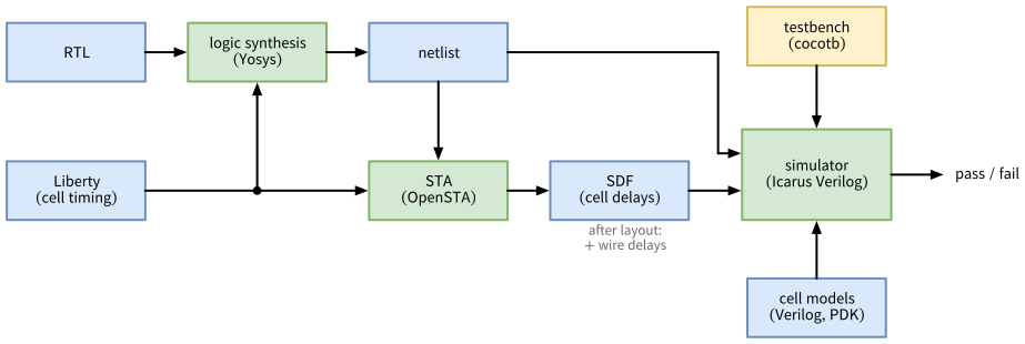
4.10.1 Without Delays
With GL=1, the runner of fifo_tb.py replaces rtl/fifo.sv by the Verilog models of the standard cells and the netlist fifo.nl.v in the folder fifo, and it works with Icarus Verilog only. It compiles with -gno-specify, which ignores the timing in the cell models, so every cell switches without delay. Synthesize the FIFO with the commands of Section 3 and run the same testbench:
cd /foss/designs/vlsi-design/content/verification/code/fifo
yosys -p "read_verilog -sv rtl/fifo.sv; synth -top fifo; \
  dfflibmap -liberty $LIB; abc -liberty $LIB; opt_clean; \
  stat -liberty $LIB; write_verilog -noattr fifo.nl.v"
cd testbenches/cocotb
GL=1 python3 fifo_tb.py
cd ../..
The netlist has 103 cells with an area of 3008 µm². Among them are 38 flip-flops of the type dfrbpq_1: 6 for the pointers and 32 for the storage, whose reset inputs are tied to 1 (Section 3.3.1). As in Section 3.4.3, the storage also needs 32 2:1 multiplexers that hold the values, and the read port 8 4:1 multiplexers. Both tests pass. As in Section 3.3.1, Icarus Verilog prints 68 sorry messages about the timing of the cell models, which do not matter without delays.
In the waveform sim_build/fifo.fst, data_o is xxxxxxxx after the reset until the first push, at gate level as at RTL, because the storage has no reset. The testbench does not fail, because the specification leaves data_o undefined while the FIFO is empty, and the scoreboard follows the specification. A testbench that compared data_o in every cycle would fail here, on a correct design.
4.10.2 With Delays from an SDF File
For a timing simulation, the cell models need the delay of every cell instance. It depends on the load and on the input slew of each instance, which only a timing analysis knows. Static timing analysis therefore writes the delays into a file in the Standard Delay Format (SDF) (IEEE 2001), and the simulator annotates them to the cell instances, a step called back-annotation. Before the layout, the SDF file holds only the delays of the cells. After the layout, it also holds the delays of the wires, computed from the extracted parasitics (Section 10).
The script syn/sta.tcl runs OpenSTA on the netlist and writes fifo.sdf. Its constraints describe the testbench: a clock period of 20 ns, and inputs and outputs that may use half a period each, because the testbench changes the inputs and samples the outputs at the falling edge. Section 6 explains these commands. For each timing path, the report of OpenSTA lists the time at which the data arrives and the time at which it is required. Their difference is the slack, and a negative slack is a timing violation. The path with the smallest slack is the critical path. Here is the entry of one flip-flop in the SDF file:
 (CELL
  (CELLTYPE "sg13cmos5l_dfrbpq_1")
  (INSTANCE _120_)
  (DELAY
   (ABSOLUTE
    (IOPATH CLK Q (0.159:0.161:0.163) (0.155:0.156:0.158))
    (IOPATH RESET_B Q () (0.000:0.000:0.000))
   )
  )
  (TIMINGCHECK
    (REMOVAL (posedge RESET_B) (posedge CLK) (-0.097:-0.097:-0.097))
    (RECOVERY (posedge RESET_B) (posedge CLK) (0.117:0.117:0.117))
    (SETUP (posedge D) (posedge CLK) (0.117:0.119:0.121))
    (SETUP (negedge D) (posedge CLK) (0.120:0.122:0.124))
    (HOLD (posedge D) (posedge CLK) (-0.062:-0.064:-0.065))
    (HOLD (negedge D) (posedge CLK) (-0.040:-0.042:-0.044))
    (WIDTH (posedge CLK) (0.217:0.217:0.217))
    (WIDTH (negedge CLK) (0.249:0.249:0.249))
    (WIDTH (negedge RESET_B) (0.000:0.000:0.000))
  )
)- Every value is a triple of a minimum, a typical, and a maximum value in ns. Here, OpenSTA computes all three from the one typical-corner library: the minimum and the maximum from its minimum and maximum analyses, and the typical value as their mean.
IOPATHis the delay from an input pin to an output pin, first for a rising and then for a falling output. The clock-to-output delay of this flip-flop is about 0.16 ns.TIMINGCHECKlists the limits that the flip-flop requires: the setup and hold times ofD, the recovery and removal times of the asynchronous reset, and the minimum pulse widths. Section 6 explains them.- The delay of a wire would be an
INTERCONNECTentry. Before the layout, these entries are all zero.
The wrapper fifo_sdf.sv instantiates the netlist and calls $sdf_annotate() at the start of the simulation. With GL=1 SDF=1, the runner uses it as the top level, compiles with -gspecify, which keeps the timing of the cell models, and passes the name of the SDF file as the run-time argument (plusarg) +SDF=...:
fifo/testbenches/cocotb/fifo_sdf.sv
// SPDX-FileCopyrightText: 2026 Simon Dorrer
// SPDX-License-Identifier: Apache-2.0
// Description: Wrapper for the timing simulation of the synthesized
// FIFO. Icarus Verilog annotates the cell delays of the SDF file that
// the plusarg +SDF=<file> names.

`default_nettype none

module fifo_sdf (
  input  wire       clk_i,
  input  wire       rst_ni,
  input  wire       push_i,
  input  wire [7:0] data_i,
  input  wire       pop_i,
  output wire [7:0] data_o,
  output wire       full_o,
  output wire       empty_o
);

  fifo u_fifo (.*);

  string sdf_file;

  initial begin
    if ($value$plusargs("SDF=%s", sdf_file)) begin
      $sdf_annotate(sdf_file, u_fifo);
    end
  end

endmodule

`default_nettype wire
sta -no_init -exit syn/sta.tcl
cd testbenches/cocotb
GL=1 SDF=1 python3 fifo_tb.py
cd ../..
The runner names the waveform after the top level, so this run writes fifo_sdf.fst and keeps the fifo.fst of the GL netlist without delays. Open either one in Surfer, and zoom in to about 1 ns around a clock edge, because the delays are only a few percent of the clock period:
surfer testbenches/cocotb/sim_build/fifo.fst
surfer testbenches/cocotb/sim_build/fifo_sdf.fst
Both tests pass. Icarus Verilog prints 38 warnings SDF WARNING: ... TIMINGCHECK not supported, one per flip-flop. It reads the delays, but it never checks a setup, hold, recovery, or removal time. A timing violation therefore shows up in Icarus Verilog only if it makes a flip-flop capture a wrong value. Simulators that support timing checks evaluate the $setuphold and $recrem checks of the cell models, and on a violation the model of the flip-flop drives its output to x, the same mechanism that VITAL, the IEEE standard for ASIC cell models in VHDL, defines.
Four traps of the open-source flow, measured with OpenSTA 3.1.0 and Icarus Verilog 14.0. sta.tcl handles the first three:
- OpenSTA writes the triples as
(min::max), without the typical value, unlesswrite_sdfgets the option-include_typ. By default, Icarus Verilog annotates the typical value, so without the option it annotates nothing, without any message. The simulation then runs without delays, while it seems to run with them. In the FIFO,empty_ofalls 0.44 ns after the clock edge that stores the first push with the typical values, and 0 ns after it without them. - Icarus Verilog reports an error for the header lines
VOLTAGEandTEMPERATURE, whose triples also lack the typical value. - Icarus Verilog annotates
INTERCONNECTentries only with the option-ginterconnect, and even then not all of those that start at a bit of an input bus that drives several cells, as each bit ofdata_idrives four. Before the layout, all wire delays are zero anyway, sosta.tclremoves allINTERCONNECTentries together with the two header lines. After the layout, the wire delays count, and the entries must stay. - Icarus Verilog does not support the state-dependent delays of the cell models, i.e., delays that depend on the values of the other inputs, e.g., the delay from the select input of a
mux2_1to its output, which depends onA0andA1. These are the 68sorry: ifnone with an edge-sensitive path is not supportedmessages. It uses the default delay of such a path instead.
The lesson of the first trap applies to every flow: zero error messages do not prove that the annotation worked. Check that a delay really shows up in the waveform.
A gate-level simulation is slower than an RTL simulation, because the netlist has more signals and events. For the small FIFO, the Python side of cocotb dominates: test_random, extended to 400 phases, i.e., 20,000 cycles, took about 1.0 s at RTL, 1.2 s at gate level, and 1.5 s with delays. For a large design, the difference grows with the number of cells, which is why only a selected set of tests runs on the netlist.
TipExercise: Timing Simulation Against Static Timing Analysis
All commands start in the folder content/verification/code/fifo. Synthesize the FIFO and write the SDF file as shown above.
- Look at the report of
sta -no_init -exit syn/sta.tcl. Which path is the critical one at 20 ns, and what limits its speed? - Find the shortest clock period at which static timing analysis reports no negative slack:
CLK_PERIOD_NS=<period> sta -no_init -exit syn/sta.tcl. The delays infifo.sdfdo not depend on the clock period. - Find the shortest clock period at which the timing simulation still passes, e.g., with 2.2, 2.0, 1.8, and 1.7 ns (command below, in the folder
testbenches/cocotb). Repeat it with other seeds. - Compare both results. Icarus Verilog checks no setup times. Is that the only reason why the timing simulation passes at clock periods for which static timing analysis reports violations? Which of the two do you trust for the tapeout?
export COCOTB_RANDOM_SEED=1
CLK_PERIOD_NS=2.2 GL=1 SDF=1 python3 fifo_tb.py
Before continuing, please finish the previous exercise. Once you are done, compare with the solution below.
TipSolution: Timing Simulation Against Static Timing Analysis
- At 20 ns, the worst slack is 8.863 ns. The critical path starts at the input
push_i, which the testbench changes at the falling edge, 10 ns after the rising one. It runs through an inverter and anor4_1, which decodes the write enable of one storage entry and drives the select inputs of its eight multiplexers. Its rising output is slow (0.66 ns): it is pulled up through four PMOS transistors in series, and it drives this load. Through amux2_1, the path then reaches theDinput of a storage flip-flop 1.01 ns after the input change, and the flip-flop needs it 0.13 ns before the clock edge (setup time). Since this path has only half a period, the period must be at least twice 1.14 ns, i.e., 2.28 ns. - At 2.28 ns, the worst slack is 0.003 ns, and at 2.27 ns, it is -0.002 ns. The other paths are faster: the slowest output,
full_o, settles 0.93 ns after the clock edge, and the slowest path between two flip-flops takes 1.75 ns plus the setup time. - The timing simulation passes at 2.2, 2.0, and 1.8 ns, with seeds 1 to 5. At 1.7 ns, it fails with every seed, already in the directed test:
data_o = XXX1XXX1, expected 00010001. The first push misses the clock edge on exactly the critical path of step 1. In the simulation, the path takes 0.89 ns from the change ofpush_ito the falling outputs of themux2_1cells, but at 1.7 ns, the next rising edge comes after 0.85 ns. Entry 0 captures the 1-bits of0x11, which arrive earlier through the faster rising outputs, keepsxin the other bits, and shows them until it is popped. - The timing simulation passes down to 1.8 ns, although static timing analysis requires 2.28 ns. The directed test does exercise the critical path, so the gap has three other causes, all in the simulator:
- Icarus Verilog checks no setup times. A flip-flop takes its
Dinput up to the clock edge, while static timing analysis requires it 0.13 ns earlier. - Icarus Verilog uses the typical value of each delay, while static timing analysis checks the setup time with the maximum values: 0.58 ns instead of 0.66 ns for the
nor4_1. - Icarus Verilog ignores the state-dependent delays of the cell models and uses the default delay from the select input of the
mux2_1to its falling output: 0.25 ns instead of 0.29 ns.
- Icarus Verilog checks no setup times. A flip-flop takes its
4.11 Choosing a Simulator
This chapter has used two simulators, and they work in very different ways. Icarus Verilog (Williams et al. 2026) is an event-driven simulator. iverilog translates the design into the vvp format, and the run-time engine vvp interprets it. Every change of a signal is an event, and the engine evaluates what depends on that signal. It knows the four values of Section 3.3, and with -gspecify, it reads the path delays in the specify blocks of the cell models. Verilator (Snyder et al. 2026) “is not a traditional simulator but a compiler”, in the words of its guide. It translates the design into C++ and fixes the order in which the logic is evaluated already when it builds the model, and a C++ compiler turns the result into a program. With --timing, it also executes the delays (#) and event controls (@) written in a testbench, but not the delays of the cell models in a GL netlist, as shown below. It knows only two values, as Section 3.3 showed.
Table 29 shows what this means for the run time. It uses a plain SystemVerilog testbench, so that no Python limits the rate. fifo_speed_tb.sv generates its stimulus itself, because $urandom differs between the simulators, and it checks the FIFO against a reference model. All four simulations pass the checks and print the same checksum, so all of them saw the same stimulus. With the netlist and the SDF file of Section 4.10, the commands are:
cd /foss/designs/vlsi-design/content/verification/code/fifo
CELLS=$PDK_ROOT/ihp-sg13cmos5l/libs.ref/sg13cmos5l_stdcell/verilog
NL="$CELLS/sg13cmos5l_udp.v $CELLS/sg13cmos5l_stdcell.v fifo.nl.v"
TB=testbenches/verilog/fifo_speed_tb.sv
verilator --binary --timing --timescale 1ns/1ps \
  --top-module fifo_speed_tb rtl/fifo.sv $TB
time ./obj_dir/Vfifo_speed_tb +CYCLES=1000000
iverilog -g2012 -o rtl.vvp rtl/fifo.sv $TB
time vvp -n rtl.vvp +CYCLES=1000000
iverilog -g2012 -gno-specify -o gl.vvp $NL $TB
time vvp -n gl.vvp +CYCLES=1000000
iverilog -g2012 -gspecify -DDUT=fifo_sdf -o sdf.vvp $NL \
  testbenches/cocotb/fifo_sdf.sv $TB
time vvp -n sdf.vvp +CYCLES=1000000 +SDF=fifo.sdffifo_speed_tb.sv. The 1,000,000 cycles are 20 ms at 50 MHz. The first build of Verilator also compiles its run-time library, which ccache keeps for the later builds. The times come from a laptop without other load and vary by about 30 % between runs, so only their ratios count.
| Simulation | Build | 1,000,000 cycles |
|---|---|---|
| Verilator, RTL | 8 s, later about 2 s | 0.4 s |
| Icarus Verilog, RTL | 0.01 s | 6 s |
| Icarus Verilog, netlist without delays | 0.02 s | 14 s |
| Icarus Verilog, netlist with SDF delays | 0.03 s | 40 s |
Three lessons follow from the table:
- Verilator pays off once a run in Icarus Verilog takes longer than the build of Verilator. Verilator runs the FIFO about 15 times faster, but after a change of the design, it first needs about 2 s to build. Both finish at the same time at about 300,000 cycles. Below that, Icarus Verilog is done first.
- The factor depends on what takes the time. Verilator gains well over 100 times on the logic of a design and on procedural code, but only about 2 times on the clock generator and the event controls of a testbench, and on this small FIFO, these take most of its run time. With 64 FIFOs, each with its own stimulus (
-GCOPIES=64for Verilator,-Pfifo_speed_tb.COPIES=64for Icarus Verilog), the factor grows to about 120, and it grows further with more FIFOs. The Verilator project states about 100 against interpreted simulators on a single thread. With cocotb, Python limits the rate of both simulators, and the exercise of Section 4.6.3 measured a factor of only 1.4, so Verilator pays off much later. - The netlist and its delays cost time. In Icarus Verilog, the netlist takes about 2.3 times as long as the RTL.
-gspecifywith the SDF delays multiplies that by about 3, and most of this comes from-gspecifyitself: without+SDF=fifo.sdf, i.e., with all delays at 0, the factor is already about 2.5. With cocotb, Python hid this cost (Section 4.10.2).
Every gate-level simulation of this course runs in Icarus Verilog, and Verilator cannot take over. Verilator ignores the timing of the cell models: it reports SPECIFYIGN for the specify blocks and for $sdf_annotate, and by default, this warning stops the build. With -Wno-SPECIFYIGN, the netlist of the FIFO builds, but even without any delays, the testbench stops in cycle 2 with wrong flags. The model of the flip-flop dfrbpq_1 takes its reset through an internal net delayed_RESET_B, which only its $recrem check drives. Verilator connects the delayed nets of $setuphold, but not this one, so the net stays 0, and all flip-flops of the netlist stay in reset. Icarus Verilog runs neither check, but it copies RESET_B to this net, and with -gspecify, its warning says so: “Delayed reference and data signals become copies of the original reference and data signals.” And even with a model that works, Verilator would hide the unknown values of Section 3.3, a main reason to simulate the netlist.
Table 30 collects the choice.
| Task | Simulator | Why |
|---|---|---|
| Lint | Verilator | --lint-only -Wall, no simulation at all |
| Short RTL runs while you design | Icarus Verilog | no build time, and it shows x |
| Long RTL runs and regressions | Verilator | speed, once an Icarus Verilog run takes longer than the build |
| Code coverage | Verilator | --coverage and verilator_coverage |
| Concurrent assertions | Verilator | Icarus Verilog does not support them (Table 28) |
| Random start values | Verilator | +verilator+rand+reset+2 with several seeds |
| Unknown values in the RTL | Icarus Verilog | four values |
| Netlist, without and with delays | Icarus Verilog | four values, and the cell models work |
The runners of this course use Icarus Verilog by default, and SIM=verilator selects Verilator. The designs of the course are small, so speed hardly matters, and a default that shows x is the safer one. Before a tapeout, run the RTL in both, Verilator with random start values: Icarus Verilog shows the x that Verilator replaces, and random values show the wrong behavior that X-optimism hides (Section 3.3.1).
4.12 Regression and Continuous Integration
A design has many tests, and every change to the RTL can break any of them. A regression runs all tests with one command and reports one verdict. In the AMS chip template (Section 1.10), make sim-all runs all simulations of a macro, at RTL and at gate level, and make regression at the top level runs lint, the simulations, the FPGA build, and the LibreLane flow of the digital example macro and of the chip, with part of the DRC skipped to save run time. Continuous integration (CI) runs the regression automatically, here on two levels. On every push to main, the template runs make regression with GitHub Actions in the latest release of the IIC-OSIC-TOOLS container (hpretl/iic-osic-tools:latest), which catches a change that breaks the design. Every night from Sunday to Thursday, IIC-OSIC-TOOLS builds its next_release branch with the newest tool versions and runs integration tests that clone the next_release branches of the templates, the chip projects, and this course, so a tool update that breaks one of them shows up the next morning, before it reaches a container release.
A regression is only useful if a failing test fails the whole command. Section 2.6.2 showed that the cocotb runner does not set the exit status when a test fails, so the runner of every testbench must check results.xml with get_results(), as all testbenches of this course do. Some more rules for a useful regression:
- Run the fast tests on every change, i.e., lint and the RTL tests. Run the slow ones every night, i.e., the gate-level and timing simulations and the complete flow.
- Use fixed seeds in the regression, so that every failure can be reproduced, and run additional random seeds every night to explore new stimuli. Always log the seed.
- Keep the regression green. A known failure hides every new one behind it.
- Turn every bug that you find into a directed test of its scenario, so that it cannot come back unnoticed.
4.13 Further Reading
- (Spear and Tumbush 2012) introduces the verification features of SystemVerilog: classes, constrained randomization, assertions, and functional coverage.
- (Bergeron 2006) covers the methodology behind testbench architectures, coverage-driven verification, and verification plans.
- The documentation of cocotb (cocotb developers 2026) describes the triggers, the runner, and the handling of signal values in detail.
- The guide of Verilator (Snyder et al. 2026) lists which language constructs it supports and which it ignores, and how to tune its speed.
- The documentation of Icarus Verilog (Williams et al. 2026) describes its compiler options and the run-time engine
vvp.
4.14 Summary
- Verification checks a design against its specification before the tapeout. Simulation works for every design at every level, but it can only show that a bug exists, never that none is left.
- A verification plan gives each feature of the specification a check and a coverage goal. The verification is complete when all checks pass and all goals are reached.
- A testbench separates the generator, the driver, the monitor, an independent reference model, the scoreboard, and the coverage collector. In cocotb, they are plain Python coroutines and classes, and the monitor samples after the driver, in the
ReadOnly()phase of the falling edge. - Exhaustive tests are possible only for small combinational blocks and small parameter values. Constrained-random tests with a logged seed, combined with directed corner values, cover the rest.
- Code coverage measures the RTL, and functional coverage measures the situations of the specification. The directed FIFO test reached 100 % line, branch, and expression coverage, but only 5 of 12 functional bins.
- Coverage measures the stimuli, and mutation testing measures the checks. A surviving mutant points to a hole in the testbench or is equivalent.
- Keep concurrent assertions in a separate checker attached with
bind, which Verilator runs. Icarus Verilog and Yosys do not support them. Keep the checks at the ports in the cocotb testbench, so that they also run on the netlist. - The same testbench runs on the netlist, without and with the delays of an SDF file. Icarus Verilog annotates the typical value of each delay by default, ignores state-dependent delays, and checks no setup or hold times, so a timing simulation is optimistic and does not replace static timing analysis.
- Icarus Verilog is an event-driven simulator with four values, and Verilator compiles the design to C++ with two values. Verilator pays off once a run in Icarus Verilog takes longer than the build of Verilator, and it also lints, measures code coverage, and checks concurrent assertions. Every gate-level simulation of this course runs in Icarus Verilog, because Verilator ignores the SDF file, keeps the flip-flop
dfrbpq_1in reset, and knows nox. - A regression runs all tests with one command and fails if any test fails, on every change and every night.
In Section 5, we look inside the synthesis step that produced the netlist of this chapter: the standard-cell library, its timing model, and the logic equivalence check that proves the netlist equivalent to the RTL without any simulation.
5 Logic Synthesis and the Standard-Cell Library
Since Section 2, we have synthesized every design with a few Yosys commands, and since Section 3, we have looked at cell areas. This chapter opens that black box. Four questions guide it. What does a synthesis tool do between the RTL and the netlist? What is a standard cell, and where do its function, its area, and its delay come from? How does a timing tool know the delay of a cell without simulating its transistors? And how do we know that the netlist still implements the RTL, without simulating it? The answers are the four steps of logic synthesis, the standard-cell library of SG13CMOS5L with its Liberty files, table-based delay calculation, PVT corners, and the logic equivalence check with EQY.
Note
All code of this chapter is available in the folder content/synthesis_lib/code of the course repository: the delay calculation in dcalc/, the scripts of the synthesis experiments in synth/, the equivalence checks in lec/, and the script that renders the cell layouts in layout/. The designs come from earlier chapters, i.e., the multiplexer of Section 2.5.4 and the barrel shifter and the FIFO of Section 4. All numbers in this chapter come from the IIC-OSIC-TOOLS image 2026.10 (Yosys 0.70, EQY 0.70, OpenSTA 3.1.0, KLayout 0.30.12) and the standard-cell libraries in the PDK of that image. Run times depend on the computer, and the ones quoted here come from a laptop. The script scripts/check_synthesis_lib.sh reproduces all other numbers: run bash scripts/check_synthesis_lib.sh in the container from the root of the repository.
For the exercises, clone the course repository into your designs folder once, if you have not done so yet:
cd /foss/designs
git clone https://github.com/iic-jku/vlsi-design.git
Define the path of the typical-corner library in every new terminal:
LIB=$PDK_ROOT/ihp-sg13cmos5l/libs.ref/sg13cmos5l_stdcell/lib
LIB=$LIB/sg13cmos5l_stdcell_typ_1p20V_25C.lib
5.1 Learning Objectives
After this chapter, you will be able to:
- describe the steps of logic synthesis from the RTL to a netlist of standard cells, and name the Yosys commands behind them
- explain what a standard cell is, how cells form rows, and which views of a library each tool of the flow reads
- read the layout of a standard cell, and compare a library of 9 tracks with one of 8 tracks
- read a Liberty file: units, cell area, pin function, timing arcs with their timing sense, and the delay and power tables
- compute the delay and the output slew of a cell by interpolation in its table, and check the result with OpenSTA
- explain process, voltage, and temperature corners, and pick the corner for a timing check
- trade area against speed in technology mapping
- explain what logic equivalence checking proves, how it matches the two designs, where it can fail falsely, and run it with EQY
5.2 What Logic Synthesis Does
Logic synthesis translates the RTL into a netlist of standard cells that implements the same function, guided by goals for area and speed. Yosys does it in four steps (Figure 26):
- Elaboration parses the RTL, builds the module hierarchy, and turns every process into a netlist of word-level cells: adders, comparators, multiplexers, and registers of any width.
always_ffbecomes a register cell, andalways_combbecomes multiplexers and logic. - Optimization works on these word-level cells. It removes constant and unused logic, detects and re-encodes state machines (
fsm), shares arithmetic between exclusive cases (share), and recognizes memories (memory). - Lowering breaks the word-level cells into generic gates and flip-flops of single bits, e.g., an 8-bit adder into its full adders, and optimizes them as a Boolean network. Yosys uses ABC (Brayton and Mishchenko 2010) for this, a tool for logic optimization from UC Berkeley.
- Technology mapping replaces the generic gates by cells of the target library:
dfflibmapthe flip-flops, and ABC the logic, now with the function, area, and delay of every cell from the Liberty file.
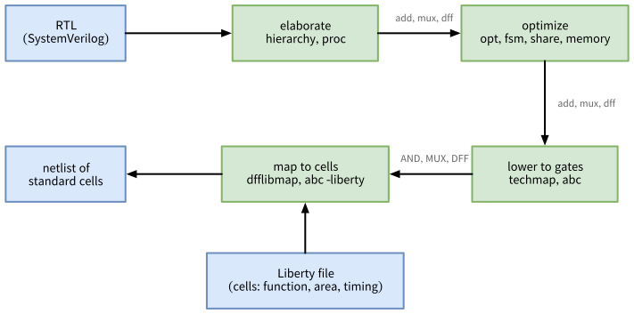
$add and $mux at the word level and $_AND_ and $_DFF_PN0_ at the gate level.
The command synth runs the first three steps. Its script, printed by yosys -p "help synth", has four stages: begin builds the hierarchy, coarse elaborates and optimizes the word-level netlist, fine lowers it to gates, and check prints the statistics. dfflibmap and abc -liberty, which follow synth in all our scripts, are the fourth step.
The multiplexer of Section 2.5.4 shows the difference between the steps. After synth alone, its eight 4:1 multiplexers and the zero flag become 67 generic gates: 40 NAND, 20 AND, 5 NOR, and 2 AND-NOT gates. After the technology mapping, they become 11 standard cells with an area of 335.7 µm²: 8 mux4_1, 2 nor4_1, and one and2_1. ABC recognized that the library has a 4:1 multiplexer cell and used it, because it is smaller and faster than the gates it replaces.
cd /foss/designs/vlsi-design/content/sv_crashcourse/code/mux4
yosys -p "read_verilog -sv rtl/mux4.sv; synth -top mux4; stat"
yosys -p "read_verilog -sv rtl/mux4.sv; synth -top mux4; \
  dfflibmap -liberty $LIB; abc -liberty $LIB; opt_clean; \
  stat -liberty $LIB"
5.3 The Standard-Cell Library
A standard cell is a small, pre-designed layout of one logic function, e.g., an inverter, a NAND gate, or a flip-flop. All cells of a library have the same height, and their widths are multiples of one site. In SG13CMOS5L, every cell is 3.78 µm high, and a site is 0.48 µm wide. The layout tool places the cells side by side in rows, where they abut and share the supply rails VDD and VSS along their top and bottom edges (Figure 27). Every second row is flipped, so that neighboring rows share a rail. This regular structure is what makes automatic placement and routing of millions of cells possible.
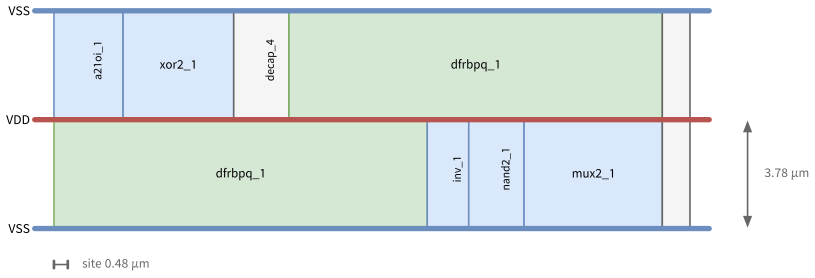
The cell names follow the pattern sg13cmos5l_<function>_<drive>. The function is a short name, e.g., inv, nand2, a21oi for an AND-OR-invert gate with a 2-input AND, mux4, or dfrbpq for a D flip-flop with an active-low reset and only a Q output. The drive strength scales the width of the transistors: a stronger cell such as inv_4 drives a larger load at the same delay, and needs more area and input capacitance for it. The library has 84 cells (Table 31). It comes from IHP, and Section 5.3.4 compares it with a second library for SG13CMOS5L.
| Category | Cells | Examples |
|---|---|---|
| combinational logic | 49 | inv_1 to inv_16, buf_1 to buf_16, nand2_1, a21oi_1, xor2_1, mux2_1, mux4_1 |
| flip-flops | 9 | dfrbpq_1, dfrbp_1, and the scan flip-flops sdfrbpq_1, sdfbbp_1 (Section 9) |
| latches | 5 | dlhq_1, dllrq_1 |
| clock gates | 2 | lgcp_1, slgcp_1 (Section 7) |
| tri-state drivers | 6 | ebufn_2, einvn_2 (Section 3.4.4) |
| delay cells | 3 | dlygate4sd1_1 to dlygate4sd3_1, for hold fixing (Section 6) |
| tie cells | 2 | tiehi, tielo, constant 1 and 0 |
| physical cells | 7 | fill_1 to fill_8, decap_4, decap_8, antennanp |
| bus holder | 1 | sighold |
The physical cells have no logic function. Fill cells close the gaps in a row, so that the wells and rails continue. Decap cells add capacitance between VDD and VSS to stabilize the supply, and the antenna diode protects transistor gates against charge collected during fabrication (Section 10).
5.3.1 Library Views
Each tool of the flow needs a different description of the same cells, called a view. The PDK keeps them in $PDK_ROOT/ihp-sg13cmos5l/libs.ref/sg13cmos5l_stdcell (Table 32).
| View | Folder | Content | Used by |
|---|---|---|---|
| Liberty | lib/ |
one file per corner: function, area, pin capacitances, delay, power | synthesis, STA, equivalence checking |
| LEF | lef/ |
size, pin shapes, and blockages of each cell, the site, and the layers | placement and routing |
| GDS | gds/ |
the full layout of each cell | the final chip layout, DRC, LVS |
| Verilog | verilog/ |
simulation models with specify blocks |
gate-level simulation (Section 4.10) |
| CDL, SPICE | cdl/, spice/ |
the transistor netlist of each cell, in the Circuit Description Language (CDL) and as SPICE | LVS, analog simulation |
| datasheet | doc/ |
one PDF per corner: function, pins, and timing in tables | the designer |
LEF (Library Exchange Format) is an abstract of the layout: placement and routing only need to know where a cell’s pins are and where the router must not place wires, not the transistors inside. The PDK also contains Xschem symbols and schematics of the cells (sym/, sch/), which let you use them in a schematic. All these views describe one fixed layout per cell, a static cell. Section 10.9.1 contrasts it with a PCell, which draws a layout from parameters.
5.3.2 The Layout of a Cell
The GDS view holds the layout of each cell, i.e., the shapes on the layers from which the masks of the chip are made. Figure 28 shows four cells of SG13CMOS5L at the same scale. Let us read the inverter inv_1 first:
- The Metal1 stripes along the bottom and the top edge are the rails VSS and VDD. They lie on the cell boundary, so that the neighboring row shares them (Figure 27).
- A transistor sits where a stripe of polysilicon (GatPoly) crosses an active area (Activ). The poly is the gate, and the active area on its two sides forms source and drain. The width of the poly stripe, 0.13 µm, is the channel length \(L\), and the height of the active area under it is the channel width \(W\).
- The NMOS transistor sits in the lower half, above VSS, with \(W\) = 0.74 µm. The PMOS transistor sits in the upper half, below VDD, inside the n-well (NWell) and under the p+ implant (pSD), with \(W\) = 1.12 µm. It is wider, because holes are less mobile than electrons. One vertical poly stripe forms both gates, and it is the input
A. - Contacts (Cont) connect the active areas and the poly to Metal1. Metal1 connects the sources to the rails and the two drains to each other, and it forms the pins
AandY. The cell uses no layer above Metal1, and the flow routes the wires between the cells on Metal2 and above (Section 10.6). - Under the rails run two active strips without a gate, the ties: an n+ strip in the n-well under VDD and a p+ strip under VSS. They connect the n-well to VDD and the p-substrate to VSS, i.e., the bulk of the PMOS and of the NMOS transistor. The n-well, the substrate, and the source and drain areas also form a parasitic thyristor. Far from a tie, a current spike can switch it on, and it then shorts the supply, which is called latch-up. A nearby tie holds the well and the substrate at their supply and keeps the thyristor off.
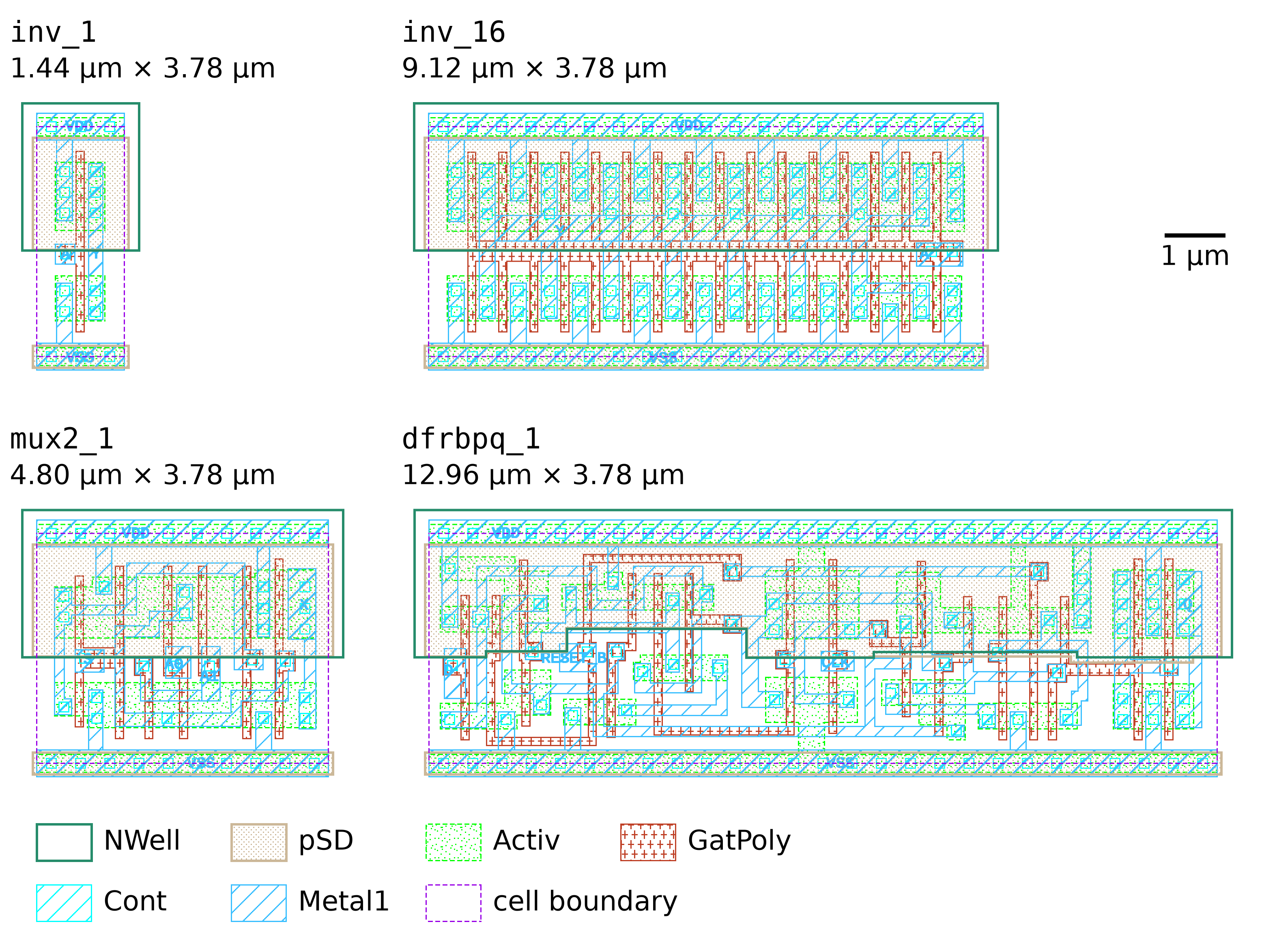
inv_1 and inv_16, the 2:1 multiplexer mux2_1, and the flip-flop dfrbpq_1, each with the size of its cell boundary (names without the prefix sg13cmos5l_). The NWell is drawn as an outline and pSD with dots, unlike in KLayout’s default, so that the transistors below them stay visible. The labels inside the cells are the pins on Metal1.
inv_16 has 16 times the transistor width of inv_1, as 16 parallel fingers of the same pair of transistors: 16 poly stripes, joined by a horizontal poly bar in the middle of the cell, with source and drain areas that neighboring fingers share. Its drive strength is 16 times that of inv_1, but its area only 6.3 times (9.12 µm against 1.44 µm wide), because the fingers share the rails, the ties, and their source and drain areas. The multiplexer mux2_1 has 12 transistors, and the flip-flop dfrbpq_1 has 32 on 27 sites, the widest of the four cells.
To look at a cell yourself, open the GDS view in KLayout with the technology of the PDK, which sets the layer colors:
GDS=$PDK_ROOT/ihp-sg13cmos5l/libs.ref/sg13cmos5l_stdcell/gds
klayout -n sg13cmos5l $GDS/sg13cmos5l_stdcell.gds
Then right-click a cell in the cell list on the left and select Show As New Top. The script layout/render_layouts.py renders the figures of this section with KLayout, all at 150 pixels per µm.
5.3.3 Gate Equivalents
Areas in µm² depend on the technology, so designers often count in gate equivalents (GE), the area divided by the area of a 2-input NAND gate. In SG13CMOS5L, nand2_1 is 1.92 µm wide and has an area of 7.2576 µm², which is 1 GE. An inv_1 is 0.75 GE, a mux4_1 5.25 GE, and the flip-flop dfrbpq_1 6.75 GE. The FIFO of Section 4, with 103 cells and 3008 µm², has 414.5 GE. A gate count in GE lets you compare designs across technologies, as long as you keep in mind that the ratios between the cells differ from library to library.
5.3.4 A Second Library with 8 Tracks
The height of a cell is usually counted in tracks, the number of horizontal routing wires that fit over it. The horizontal layers of SG13CMOS5L, Metal1 and Metal3, have a pitch of 0.42 µm, the distance from the center of one wire to the center of the next, and 3.78 µm are 9 × 0.42 µm. The cells of SG13CMOS5L are therefore 9-track cells. The vertical layers Metal2 and Metal4 have a pitch of 0.48 µm, the width of a site. Fewer tracks give smaller cells, but leave less room for the transistors and for the wires inside a cell.
The PDK in the image holds a second library for the same thin-oxide transistors, version 1.1 of EZ130 8T from ETH Zurich (Castañeda et al. 2026). Students designed its cells in a course on standard-cell design at ETH Zurich, and it was released as open source in 2026. Its cells are 3.36 µm high, 8 tracks of 0.42 µm, on a site of 0.42 µm (Table 33). Their names carry no prefix: INVX1 is an inverter of drive strength X1, and P5 stands for one half, e.g., X1P5 for 1.5. A third library, sg13cmos5l_stdcell_hv, uses thick-oxide transistors for 3.3 V, and its cells are 7.14 µm high, 17 tracks. In short, the three are IHP LV, ETH LV, and IHP HV, for low and high voltage. The rest of this book uses IHP LV.
| Category | Cells | Examples |
|---|---|---|
| combinational logic | 152 | INVX1 to INVX64, BUFX1 to BUFX64, NAND2X1, AOI21X1, XOR2X1, MUX2X1, MUX4X1, the full adder FAX1 |
| flip-flops | 27 | DFFQX1 without reset, DFFRQX1, the banks DFFRQ2X1 and DFFRQ4X1, the scan flip-flop DFFMRQX2 |
| latches | 14 | LATQX1, LATNRX1 |
| clock gates | 7 | CGX1, CGTSX1 |
| tri-state drivers | 4 | TBUFX1, TINVX1 |
| delay cells | 1 | DLY1X2 |
| tie cells | 2 | TIEHI, TIELO |
| physical cells | 13 | FILLER1 to FILLER16, DECAP4 to DECAP32, ANTENNA2 to ANTENNA8, WELLTAP |
| bus holder | 0 | none |
The Liberty files describe 214 of the cells, all except the five fill cells and WELLTAP, which have neither a function nor a timing. Compared with IHP LV, five differences matter for the flow:
- Area. For the same function and drive strength, a cell of ETH LV is smaller: the inverter
INVX3needs 4.23 µm² against 5.44 µm² forinv_1, and the flip-flop with resetDFFRQX328.22 µm² against 48.99 µm² fordfrbpq_1. In the gate equivalents of its own library, withNAND2X1at 5.6448 µm²,DFFRQX1has 5 GE against the 6.75 GE ofdfrbpq_1, an example of the different ratios of Section 5.3.3. On eight synthesis benchmarks, its authors report a significantly smaller area than with IHP’s library of SG13G2, which has the same cells as IHP LV, at a competitive timing (Castañeda et al. 2026). - Choice. ETH LV has 220 cells against 84: 13 buffers from
BUFX1toBUFX64against 5, the full adderFAX1and the half adderHAX2, complex gates with inverted inputs such asAOI21BX1, flip-flops without reset such asDFFQX1, which IHP LV lacks (Section 3.3.1), and flip-flop banks that store 2 or 4 bits with one clock and one reset,DFFRQ2X1andDFFRQ4X1. The 4-bit banks are the only cells of double height, 6.72 µm over two rows. Yosys maps each register bit to a flip-flop of its own, so the banks stay unused in the open-source flow. - Drive strength. The digit counts the drive in units of the library’s own X1, and X1 is three times weaker than
_1in IHP LV:INVX3has themax_capacitanceofinv_1, 0.3 pF, andINVX1only 0.1 pF.INVX1,INVX2, andINVX3even share one footprint (Figure 29). ETH LV makes a cell weaker by narrowing its transistors, with an NMOS and a PMOS width of 0.30 µm and 0.48 µm inINVX1against 0.86 µm and 1.32 µm inINVX3, while IHP LV keeps the transistors ofinv_1and adds fingers (Figure 28). When a design moves from one library to the other, a cell that a script or a constraint names must be replaced by the cell with the samemax_capacitance, not by the one with the same digit. - Ties. The cells of ETH LV have no ties: each inverter in Figure 29 has two active areas, its two transistors, where
inv_1has four. The ties sit in a separate cell,WELLTAP, with an n+ strip in the n-well and a p+ strip above VSS. The layout rules of SG13CMOS5L demand a tie within 20 µm of every transistor (rulesLU.aandLU.b), so the flow must place aWELLTAPin every row at regular distances, which IHP LV does not need (Section 10.3). - Corners and views. ETH LV is characterized for 1.2 V only, at the three corners
tt_1p20v_25c,ss_1p08v_125c, andff_1p32v_m40c, against the six corners of IHP LV at 1.2 V and 1.5 V (Section 5.6). It comes with Liberty, LEF, GDS, Verilog, and CDL views, but without SPICE netlists and Xschem symbols. The image installs it in the tree of SG13G2,$PDK_ROOT/ihp-sg13g2/libs.ref/ez130_8t, with a technology LEF for each of the two PDKs, since both have the same transistors and the same layers up to Metal1. The PDK has no LibreLane configuration for it, so a macro on ETH LV must name all views in its own configuration.
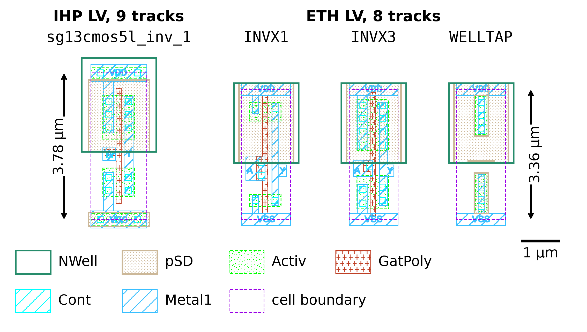
inv_1 of IHP LV against the inverters INVX1 and INVX3 and the tap cell WELLTAP of ETH LV, at the same scale and in the colors of Figure 28. The arrows give the heights of the cell boundaries. INVX3 has the drive strength of inv_1, and INVX1 a third of it in the same footprint. The ETH cells have no ties under their rails. WELLTAP holds them: an n+ strip in a gap of the pSD inside the n-well, and a p+ strip above VSS.
Rows of different height cannot abut, so a macro uses one library. ETH LV offers smaller cells and more of them, IHP LV the simpler flow, which is why the exercises of this book use it.
5.4 Inside a Liberty File
The Liberty format (.lib), introduced by Synopsys and freely available, is the de-facto standard that describes the logic, timing, and power of every cell in plain text. The header of a library defines the units and the conditions of the characterization:
library (sg13cmos5l_stdcell_typ_1p20V_25C) {
  delay_model : table_lookup;
  capacitive_load_unit (1,pf);
  leakage_power_unit : "1pW";
  time_unit : "1ns";
  ...
  input_threshold_pct_rise : 50;
  nom_process : 1;
  nom_temperature : 25;
  nom_voltage : 1.2;
  output_threshold_pct_rise : 50;
  slew_lower_threshold_pct_rise : 20;
  slew_upper_threshold_pct_rise : 80;
  ...
Times are in ns and capacitances in pF. A delay, the propagation delay \(t_\text{pd}\) of the cell, is measured from 50 % of the input swing to 50 % of the output swing, and a slew (transition time) from 20 % to 80 % of the swing. The library also defines templates for its tables. In the template of the delay tables, index_1 is the input slew and index_2 is the total load capacitance at the output, with seven values each. Here is the inverter inv_1, shortened to the parts that matter:
cell (sg13cmos5l_inv_1) {
  area : 5.4432;
  cell_leakage_power : 63.0032;
  pin (Y) {
    direction : "output";
    function : "!(A)";
    max_capacitance : 0.3;
    timing () {
      related_pin : "A";
      timing_sense : negative_unate;
      timing_type : combinational;
      cell_rise (TIMING_DELAY_7x7ds1) {
        index_1 ("0.0186, 0.0966, 0.174, 0.3294, ...");
        index_2 ("0.001, 0.0234, 0.039, 0.0648, ...");
        values ( \
          "0.0205647, 0.0848969, 0.128137, ...", \
          ...);
      }
      rise_transition (TIMING_DELAY_7x7ds1) { ... }
      cell_fall (TIMING_DELAY_7x7ds1) { ... }
      fall_transition (TIMING_DELAY_7x7ds1) { ... }
    }
    internal_power () { ... }
  }
  pin (A) {
    direction : "input";
    max_transition : 2.5074;
    capacitance : 0.00286745;
  }
}areais the cell area in µm², andcell_leakage_powerthe static power in pW. The full file also lists the leakage per input state, 82.5 pW forA= 1 and 43.5 pW forA= 0, and the cell value is their average.functiongives the Boolean function of the output. Synthesis maps logic with it, and the equivalence check of Section 5.8 reads it.capacitanceof an input pin is the load it presents to its driver, here 2.87 fF.max_capacitanceis the largest load the output may drive, 0.3 pF, andmax_transitionthe largest slew an input may see, 2.51 ns, the last slew index of the tables.- A
timinggroup describes one timing arc from the related pin (related_pin) to the pin whose group contains it, here from the inputAto the outputY.timing_typesays what kind of arc it is:combinationalfor logic, and for a flip-flop, e.g.,rising_edgefrom the clock toQ,setup_risingandhold_risingfor the timing checks ofD, andrecovery_risingandremoval_risingfor its asynchronous reset. timing_senseis the unateness of the arc. Apositive_unatearc (AND, OR, buffer) turns a rising input into a rising output, anegative_unatearc (NAND, NOR, inverter) into a falling one, and anon_unatearc (XOR, the select input of a multiplexer, the clock of a flip-flop) can do either, depending on the other inputs.- Four 7×7 tables give the delay (
cell_rise,cell_fall) and the output slew (rise_transition,fall_transition) for a rising and a falling output, andinternal_powergives the energy of a switching event in the same form.
A flip-flop adds a group that defines its state, here for dfrbpq_1:
ff (IQ,IQN) {
  clear : "!RESET_B";
  clocked_on : "CLK";
  next_state : "D";
}
The internal state IQ takes the value of D at the rising edge of CLK and is cleared while RESET_B is low, and the function of the output Q is "IQ". The setup and hold times of D are tables as well, with 4×4 entries over the slews of the data and the clock signal. Section 6 uses them.
5.5 Delay Calculation with Tables
Old libraries modeled a delay as a constant plus a resistance times the load, which is fine for long-channel transistors. In modern technologies, the delay depends on both the load and the input slew, and the slew also changes how the delay grows with the load (Figure 30). For a fast input edge, the delay of inv_1 grows almost linearly with the load, but a slow edge bends the curve at small loads. No simple formula fits this, so the library stores the delay as a table over both, the nonlinear delay model (NLDM). Advanced nodes add current-source models, the composite current source (CCS) and the effective current source model (ECSM), for even more accuracy, but the SG13CMOS5L libraries contain NLDM tables only.
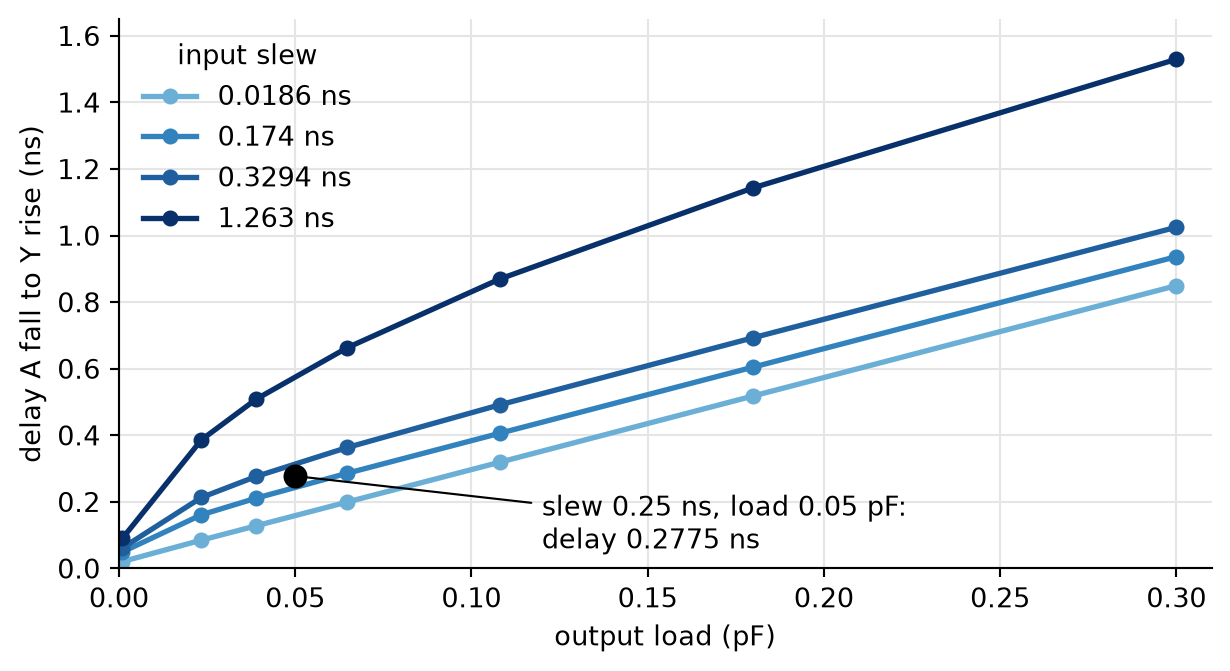
cell_rise of sg13cmos5l_inv_1 in the typical library: the delay from a falling input A to a rising output Y over the output load, for four of the seven input slews of the table. The markers are the table entries. The delay grows with the load and with the input slew. For a fast input, it grows almost linearly with the load, while a slow input bends the curve at small loads. The black point is the operating point of Section 5.5, an input slew of 0.25 ns and a load of 0.05 pF, which lies between the table entries and gives 0.2775 ns by interpolation.
A timing tool computes the delay of each cell instance from two values: the slew at its input, which the driving cell determines, and the load at its output, i.e., the sum of the input capacitances of all driven pins plus the capacitance of the wire. The two values rarely coincide with table indices, so the tool interpolates linearly between the four neighboring entries, first along the load and then along the slew.
Take an inv_1 with an input slew \(s = 0.25\) ns and a load \(C = 0.05\) pF, and compute its delay for a rising output. The neighbors in cell_rise are at the slews 0.174 and 0.3294 ns and the loads 0.039 and 0.0648 pF:
cell_rise of inv_1 around \(s\) = 0.25 ns and \(C\) = 0.05 pF
| \(C\) = 0.039 pF | \(C\) = 0.0648 pF | |
|---|---|---|
| \(s\) = 0.174 ns | 0.211237 ns | 0.285953 ns |
| \(s\) = 0.3294 ns | 0.276414 ns | 0.363301 ns |
The position between the indices is \(u = (0.05 - 0.039)/(0.0648 - 0.039) = 0.4264\) along the load and \(v = (0.25 - 0.174)/(0.3294 - 0.174) = 0.4891\) along the slew. Interpolating both rows along the load gives \(0.211237 + u \cdot 0.074716 = 0.2431\) ns and \(0.276414 + u \cdot 0.086887 = 0.3135\) ns, and interpolating between them along the slew gives the delay
\[t_\text{pd} = 0.2431 + v \cdot (0.3135 - 0.2431) = 0.2775 \text{ ns.}\]
OpenSTA shows this calculation with report_dcalc, including the four table entries it used (v is a falling and ^ a rising edge):
A v -> Y ^
P = 1.0000 V = 1.2000 T = 25.0000
------- input_net_transition = 0.2500
|       total_output_net_capacitance = 0.0500
|        0.0390     0.0648
v      --------------------
0.1740 | 0.2112     0.2860
0.3294 | 0.2764     0.3633
Table value = 0.2775
PVT scale factor = 1.0000
Delay = 0.2775
The output slew comes from rise_transition in the same way, and it becomes the input slew of the next cell. A path delay is therefore computed stage by stage, from the inputs to the outputs: a slow edge makes the next cell slow as well.
The load includes the capacitance of the wires, which is unknown before the layout. The SG13CMOS5L libraries contain 12 wire-load models, which estimate a wire’s capacitance from the number of loads it drives (its fanout) and the size of the design. OpenSTA uses them only when you select one with set_wire_load_model. The model 1k, for example, estimates 0.0182 pF for a net with eight loads, as much as the inputs of six inv_1 cells. Without it, as in all timing analyses of this book so far, the pre-layout delays include no wires. In the LibreLane flow, the wire capacitances are estimated from the placement and later extracted from the routed layout (Section 10).
TipExercise: Interpolate a Delay Table
All commands start in the folder content/synthesis_lib/code/dcalc. The netlist one_inv.v holds one inv_1, and dcalc.tcl runs report_dcalc on it. The environment variables SLEW (in ns) and LOAD (in pF) set the input slew and the output load.
- Find the inverter
sg13cmos5l_inv_4in the typical library (less $LIB, then search with/inv_4). What is its area in gate equivalents? What is the input capacitance ofA, and what is the largest load thatYmay drive? Compare the three values with those ofinv_1. - Compute by hand the delay of
inv_1from a rising input to a falling output (cell_fall) at an input slew of 0.25 ns and a load of 0.05 pF. - Check your result with OpenSTA:
sta -no_init -exit dcalc.tcl. What is the output slew of the falling edge? - Run the analysis with a load of 0.4 pF:
LOAD=0.4 sta -no_init -exit dcalc.tcl. Which table entries does OpenSTA use now, and what does it report at the end? - Replace the
inv_1by aninv_4withsed -i 's/inv_1/inv_4/' one_inv.v, and run the analysis with a load of 0.2 pF:LOAD=0.2 sta -no_init -exit dcalc.tcl. Compare the delays with those ofinv_1at 0.05 pF. Restore the netlist withgit restore one_inv.v.
Before continuing, please finish the previous exercise. Once you are done, compare with the solution below.
TipSolution: Interpolate a Delay Table
- The area of
inv_4is 10.8864 µm², i.e., 10.8864 / 7.2576 = 1.5 GE, twice the area ofinv_1. The input capacitance ofAis 0.0112 pF, 3.9 times the 0.00287 pF ofinv_1, andmax_capacitanceofYis 1.2 pF, four times the 0.3 pF ofinv_1. - The neighbors in
cell_fallare 0.196172 and 0.259858 ns at the slew 0.174 ns, and 0.259958 and 0.33725 ns at 0.3294 ns. With \(u = 0.4264\) and \(v = 0.4891\) as in the text, the rows give 0.2233 and 0.2929 ns, and the delay is \(0.2233 + v \cdot (0.2929 - 0.2233) = 0.2574\) ns. - OpenSTA reports
A ^ -> Y vwithTable value = 0.2574and an output slew of 0.1981 ns. The falling output is faster than the rising one (0.2775 ns), because the NMOS transistor of the inverter is stronger than the PMOS transistor. - The load of 0.4 pF lies beyond the last load index of 0.3 pF. OpenSTA uses the rows of the slews 0.174 and 0.3294 ns as before, and extrapolates linearly from the two last columns, 0.18 and 0.3 pF: the rising delay grows to 1.2563 ns. At the end,
report_check_typesreports a violation ofmax capacitance: the limit is 0.3 pF, the load 0.4 pF, and the slack -0.10 pF. An extrapolated value is a guess, which is why the library limits the load: the flow must insert a buffer or use a stronger cell. - At 0.2 pF,
inv_4has a falling delay of 0.2578 ns and a rising delay of 0.2771 ns, the same within 0.4 ps asinv_1at 0.05 pF. Four times the drive strength gives the same delay at four times the load. The price is twice the area and almost four times the input capacitance, which in turn loads the cell that drivesinv_4.
5.6 Corners
The speed of a transistor depends on the fabrication process, the supply voltage, and the temperature (PVT). A chip must work for every combination it will see, so the library is characterized at several corners. A fast corner combines fast transistors, a high supply voltage, and a low temperature. A slow corner combines slow transistors, a low supply voltage, and a high temperature. A typical corner lies in between. SG13CMOS5L has six Liberty files sg13cmos5l_stdcell_<corner>.lib, three for a nominal supply of 1.2 V and three for 1.5 V (Table 35).
inv_1 at an input slew of 0.25 ns and a load of 0.05 pF
| Corner | Process | Voltage | Temperature | Fall delay | Rise delay |
|---|---|---|---|---|---|
fast_1p32V_m40C |
fast | 1.32 V | -40 °C | 0.197 ns | 0.205 ns |
typ_1p20V_25C |
typical | 1.20 V | 25 °C | 0.257 ns | 0.278 ns |
slow_1p08V_125C |
slow | 1.08 V | 125 °C | 0.353 ns | 0.376 ns |
fast_1p65V_m40C |
fast | 1.65 V | -40 °C | 0.145 ns | 0.154 ns |
typ_1p50V_25C |
typical | 1.50 V | 25 °C | 0.188 ns | 0.208 ns |
slow_1p35V_125C |
slow | 1.35 V | 125 °C | 0.259 ns | 0.276 ns |
At 1.2 V, the same inverter is about 1.8 times slower in the slow corner than in the fast one. Each timing check is usually hardest to meet in one corner: the setup check, which limits the clock frequency, with the maximum delays of the slow corner, and the hold check with the minimum delays of the fast corner (Section 6). For the signoff before a tapeout, both checks run in all corners, because the clock network slows down with the logic, and a hold violation can also appear in the slow corner. Older libraries had a single table and scaled it to other conditions with derating factors. Today, every corner is characterized on its own, because the scaling is not linear.
5.7 Synthesis with Yosys in Practice
The command sequence that we have used since Section 3 maps a design onto SG13CMOS5L:
yosys -p "read_verilog -sv rtl/fifo.sv; synth -top fifo; \
  dfflibmap -liberty $LIB; abc -liberty $LIB; opt_clean; \
  stat -liberty $LIB; write_verilog -noattr fifo.nl.v"
read_verilog -svreads the SystemVerilog source, andsynth -top fiforuns elaboration, optimization, and lowering withfifoas the top module.dfflibmap -liberty $LIBmaps the generic flip-flops onto the flip-flops of the library. IHP LV has no flip-flop without a reset, so a register without reset becomes adfrbpq_1with its reset input tied to 1 (Section 3.3.1).abc -liberty $LIBmaps the logic onto the cells of the library, with their functions, areas, and delays.opt_cleanremoves unused wires and cells,stat -liberty $LIBprints the cell counts and the total cell area, andwrite_verilog -noattrwrites the netlist without Yosys attributes.
ABC can map the same logic for a small area or for a short delay. With -constr <file>, ABC appends buffering and gate sizing to its mapping: it inserts buffers into nets with a large fanout, and it resizes cells, stronger ones on the slowest paths and weaker ones elsewhere (buffer, upsize, dnsize). For the delays, it needs the cell that drives the inputs and the load of the outputs, which the file sets. The file synth/abc.constr sets an inv_2 as driver and a load of 10 fF (the unit is fF here), the 0.01 pF of the timing scripts of this chapter. The option -D <ps> sets a delay target in picoseconds for the sizing. Without -constr, -D has no effect on the barrel shifter of the next exercise. The option -script replaces ABC’s default commands, e.g., by the area-only mapping amap.
In the LibreLane flow, the variable SYNTH_STRATEGY selects one of nine prepared ABC scripts, AREA 0 to AREA 3 and DELAY 0 to DELAY 4. The default is AREA 0, and the counter of the AMS chip template uses DELAY 4. Which strategy wins depends on the design, so the only reliable way to choose is to try several and compare the timing reports.
TipExercise: Area Against Delay
All commands start in the folder content/synthesis_lib/code/synth. The 32-bit barrel shifter of Section 4 is a large block of multiplexers, which makes the effect of the mapping visible.
Synthesize the barrel shifter with
WIDTH = 32three times, with the default mapping, with a delay target of 1 ns, and with the area mapping. Each time, note the number of cells and the area, and write the netlist tobarrel_shift.nl.v:yosys -p "read_verilog -sv \ ../../../verification/code/barrel_shift/rtl/barrel_shift.sv; \ chparam -set WIDTH 32 barrel_shift; synth -top barrel_shift; \ abc -liberty $LIB; opt_clean; \ stat -liberty $LIB; write_verilog -noattr barrel_shift.nl.v"For the delay target, replace the
abccommand byabc -D 1000 -constr abc.constr -liberty $LIB, and for the area mapping byabc -liberty $LIB -script +strash;dch,-f;amap;topo.After each synthesis, find the longest path with
TOP=barrel_shift sta -no_init -exit comb_sta.tclin the typical corner, and withCORNER=slow_1p08V_125C TOP=barrel_shift sta -no_init -exit comb_sta.tclin the slow corner. The columnActual Delaygives the delay of the slowest path from an input to an output.Collect the results in a table. How much area does the fastest version cost compared with the smallest? Which version would you choose for a block that has to run at 250 MHz, and which for one that runs at 50 MHz? Which corner decides?
Repeat the delay-targeted mapping with 3000 ps, with 500 ps, and with
-constr abc.constrbut without-D. What happens, and why can a delay target not be met by mapping alone?
Before continuing, please finish the previous exercise. Once you are done, compare with the solution below.
TipSolution: Area Against Delay
The default mapping gives 747 cells and 9399.0 µm², the delay target of 1 ns 818 cells and 10,030.4 µm², and the area mapping 765 cells and 7305.5 µm².
The longest paths are 2.51 ns with the default mapping, 1.50 ns with the delay target, and 4.81 ns with the area mapping in the typical corner, and 3.87, 2.33, and 7.36 ns in the slow corner.
The results:
Mapping Cells Area Typical Slow amap(area)765 7305.5 µm² 4.81 ns 7.36 ns default 747 9399.0 µm² 2.51 ns 3.87 ns -D 1000 -constr818 10,030.4 µm² 1.50 ns 2.33 ns The fastest version needs 37 % more area than the smallest and is 3.2 times faster. The slow corner decides, because it limits the setup check (Section 5.6). At 250 MHz, a period of 4 ns, the delay-targeted mapping leaves 1.67 ns for the registers around the block. The default mapping leaves only 0.13 ns, too little for the clock-to-output delay and the setup time of the flip-flops (Section 6). At 50 MHz, 20 ns, even the area mapping is fast enough, and it saves 22 % of the area of the default mapping.
With 3000 ps, the netlist has 818 cells, 9914.3 µm², and a longest path of 1.88 ns. The sizing stops as soon as the target is met and saves 116 µm². With 500 ps and without
-D, the result is the same as with 1000 ps: 10,030.4 µm² and 1.50 ns. The target only limits the sizing, and below 1.50 ns, the sizing finds nothing faster. ABC restructures the logic only locally and picks and sizes the cells of the library. A much faster block needs a different architecture, e.g., fewer logic levels or a pipeline register (Section 7).
5.8 Logic Equivalence Checking
The netlist must implement the RTL, but why should we believe that it does? Synthesis is a large program with bugs of its own, settings and scripts can change the function, the netlist can be edited by hand after synthesis (an engineering change order, ECO), and a netlist can simply be stale, i.e., synthesized from an older version of the RTL. A gate-level simulation with the testbench of the RTL checks the netlist for the stimuli it applies (Section 4.10). A logic equivalence check (LEC) proves for every input that the netlist computes the same function as the RTL, without any stimulus and without any timing.
Figure 31 shows the idea of a classic equivalence checker, such as the commercial tools of the industry. The checker reads both designs: the reference, called gold, which is the RTL, and the implementation, called gate, which is the netlist. It matches the registers and outputs of both sides by name. The matched registers are cut points: they cut both designs into combinational cones, and the output of a matched register becomes a free input of the cones behind it, an input that the solver may set to any value, but to the same value on both sides. For every cone, the checker then proves with a formal solver that gold and gate compute the same function of the cone’s inputs. If every cone agrees, the two designs are equivalent from any state, which is a stronger statement than any simulation can make.
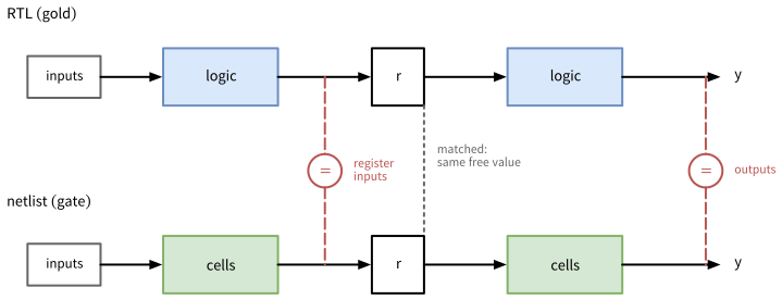
This works because synthesis keeps the registers and their names. It fails falsely where synthesis changes the registers: when it re-encodes a state machine (the same name now holds a one-hot instead of a binary code), moves logic across registers (retiming), or merges or duplicates registers. A checker then needs extra rules to match the registers, or a sequential equivalence check (SEC), which starts both designs from reset and compares them over time without matching registers, at a much higher cost. Equivalence checking runs after every step that changes the netlist: after synthesis, after place and route (which adds buffers, the clock tree, and hold cells), after the insertion of scan chains (Section 9), and after every ECO. It has clear limits: it does not see timing, it does not see the start values of registers without reset (Section 3.3), and it proves the netlist equal to the RTL, not the RTL correct.
5.8.1 EQY
EQY (YosysHQ 2026a) is the equivalence checker of the Yosys suite. A configuration file describes gold and gate as Yosys scripts and selects a strategy for the proofs. Here is the check of the FIFO of Section 4:
lec/fifo.eqy
# SPDX-FileCopyrightText: 2026 Simon Dorrer
# SPDX-License-Identifier: Apache-2.0
# Description: Equivalence check of the FIFO of chapter 4: its RTL
# (gold) against the synthesized netlist fifo.nl.v (gate). Run in this
# folder with stdcell.lib linked to the typical library of SG13CMOS5L:
# eqy -f -d fifo_eqy fifo.eqy

[gold]
# slang reads the RTL with another frontend than synthesis did
plugin -i slang
read_slang ../../../verification/code/fifo/rtl/fifo.sv --top fifo
hierarchy -check -top fifo
proc
# slang keeps mem_q as a memory, synthesis made it registers
memory_map
flatten -noscopeinfo

[gate]
# The cell functions come from the Liberty file
read_liberty -ignore_miss_func stdcell.lib
read_verilog fifo.nl.v
hierarchy -check -top fifo
flatten -noscopeinfo
# Fails if a cell had no model and stayed a black box
select -assert-none t:sg13cmos5l_*

[collect *]
# full_o and empty_o also feed logic inside the FIFO: compare them
# together with that logic instead of cutting it there
bind full_o
bind empty_o

[strategy sby]
use sby
engine abc pdr
[gold]reads the RTL with slang (Popoloski 2026), a different SystemVerilog frontend from the one that synthesis used. If both sides went through the same frontend, a misreading of the RTL would end up in both, and the check would pass. slang keeps the storage arraymem_qas a memory, while synthesis turned it into registers, somemory_mapturns it into registers on the gold side as well.[gate]reads the netlist and takes the function of every cell from the Liberty file, linked asstdcell.lib.-ignore_miss_funcskips cells with an output that has no function, such as the clock gatelgcp_1, whichread_libertywould otherwise refuse. The two checks make sure that no cell escapes the comparison:hierarchy -checkfails if the netlist uses a cell that was skipped, andselect -assert-nonefails if any cell is still a black box afterflatten. They turn a missing or skipped cell model into a clear error at once, instead of an obscure error later in the run.[collect *]withbindis explained below.[strategy sby]proves each partition (see below) with the formal tool SymbiYosys and the PDR engine of ABC (property-directed reachability).
Synthesize the FIFO into the folder lec, link the library, and run EQY:
cd /foss/designs/vlsi-design/content/synthesis_lib/code/lec
ln -sf $LIB stdcell.lib
yosys -p "read_verilog -sv \
  ../../../verification/code/fifo/rtl/fifo.sv; synth -top fifo; \
  dfflibmap -liberty $LIB; abc -liberty $LIB; opt_clean; \
  write_verilog -noattr fifo.nl.v"
eqy -f -d fifo_eqy fifo.eqy
EQY prints Successfully proved designs equivalent and DONE (PASS, rc=0) after about 3 s. The matched names are in fifo_eqy/matched.ids. A failing check exits with status 2 and names the partitions it could not prove.
EQY works in a way related to Figure 31, but not identical. It splits the designs into partitions, by default one per matched register or output, usually with all bits of a signal together. A matched signal that another partition computes becomes a free input, i.e., a cut point, while the registers of a partition stay inside it. The [collect *] section holds commands that change the partitions, for all modules (*). Here, it merged them into 3 partitions, listed in fifo_eqy/partition.list. Because a partition keeps its registers, the strategy sby proves it over time: SymbiYosys shows with PDR that gold and gate agree at the matched signals in every cycle. The registers of the netlist start with any value, those of the RTL start unknown (x), and an x on the gold side matches any value on the gate side. EQY therefore proves the netlist equal to the RTL in every state that the RTL can reach after its reset, not from any state like a classic checker. A state that the reset never reaches is not compared, and a register of the RTL without reset is only checked once it holds a known value.
5.8.2 A False Failure
Without the [collect *] section, EQY reports a failure: it cannot prove 5 of the 9 partitions, among them the write pointer. For each failed partition, the solver writes a counterexample, a waveform of input values for which gold and gate differ. The counterexample in strategies/fifo.wr_ptr_q/sby/fifo.wr_ptr_q/engine_0/trace.vcd of the work folder, opened in Surfer, shows why. The partition of wr_ptr_q has the free inputs push_i, full_o, and rd_ptr_q, among others. After the reset, wr_ptr_q is 000, and the solver sets push_i to 1, full_o to 0, and rd_ptr_q to 100. Gold increments wr_ptr_q to 001, while the gate side keeps 000.
The reason is a cut point. In the RTL, the push logic reads the flag full_o, an output that EQY matched, so the gold partition reads the free input full_o. The netlist does not read the output net: synthesis computes “full” a second time inside the push logic, from the pointers, so the gate partition reads the free input rd_ptr_q instead. Nothing ties the two free inputs together, and the solver picks values that no real circuit can produce: with the pointers 000 and 100, the FIFO is full, but full_o is 0. The partitions differ, the designs do not.
bind full_o puts the registers that read full_o, the write pointer and the storage, into the partition of full_o, and bind empty_o puts the read pointer into the partition of empty_o. The logic that computes a flag then stays together with the logic that reads it, instead of being cut at the output net, and the check passes. Two lessons follow. A failing partition is not yet a bug: read the counterexample and decide whether a real circuit can be in that state. And a check that passes must also be able to fail, since a check that is set up wrongly, e.g., with a skipped cell model or a black box, would pass for any netlist. With the RTL changed after synthesis, e.g., to accept a push into a full FIFO during a pop (mutant M3 of Section 4.9), the same configuration fails in the partition full_o, as it must.
Other equivalence checkers exist. kepler-formal, also in the image, compares two designs either combinationally (LEC) or sequentially from reset (SEC). The commercial tools Cadence Conformal and Synopsys Formality are the standard in industry. LibreLane has an equivalence step with EQY as well, but it prepares the cell models only for the sky130 PDK, so we run EQY ourselves.
TipExercise: Prove It, Break It
All commands start in the folder content/synthesis_lib/code/lec. Link the library with ln -sf $LIB stdcell.lib, if you have not done so for the FIFO. The folder holds the reference solution barrel_shift.eqy, so move it out of the way first: mv barrel_shift.eqy barrel_shift_solution.eqy.
Sketch gold and gate of the barrel shifter in the style of Figure 31. Where are the cut points, and how many cones do you expect?
Synthesize the barrel shifter with
WIDTH = 32and the default mapping intobarrel_shift.nl.vin this folder, with the same command as in the previous exercise. How many cells does the netlist have?Write
barrel_shift.eqyafter the example offifo.eqy. Which parts of the FIFO configuration does the barrel shifter not need, and why? Note that slang takes a parameter as-G WIDTH=32.Run
eqy -f -d bs_eqy barrel_shift.eqy. How many partitions does EQY build? Does the number match your sketch?Break the netlist: replace the first
sg13cmos5l_a21oi_1by ansg13cmos5l_o21ai_1, which has the same pins and a different function:cp barrel_shift.nl.v barrel_shift_good.nl.v sed -i '0,/sg13cmos5l_a21oi_1 /s//sg13cmos5l_o21ai_1 /' \ barrel_shift.nl.v eqy -f -d bs_mut barrel_shift.eqyOpen the counterexample
bs_mut/strategies/*/sby/*/engine_0/trace.vcdin Surfer. The signals__pi_*are the inputs, and__po_*__goldand__po_*__gatethe outputs of both sides. Which input vector shows the difference, and which output bit differs? Compute the correct output by hand.
Before continuing, please finish the previous exercise. Once you are done, compare with the solution below.
TipSolution: Prove It, Break It
The barrel shifter has no registers, so the only matched points are its inputs and its output
data_o. Both lanes of the sketch hold one cone, from the inputs todata_o, with no cut point inside.The netlist has 747 cells, as with the default mapping of the previous exercise.
The barrel shifter has no storage array and no output that it reads internally, so it needs neither
memory_mapnor[collect *]:
lec/barrel_shift.eqy
# SPDX-FileCopyrightText: 2026 Simon Dorrer
# SPDX-License-Identifier: Apache-2.0
# Description: Equivalence check of the 32-bit barrel shifter of
# chapter 4: its RTL (gold) against the synthesized netlist
# barrel_shift.nl.v (gate). Run in this folder with stdcell.lib linked
# to the typical library of SG13CMOS5L:
#   eqy -f -d bs_eqy barrel_shift.eqy

[gold]
plugin -i slang
read_slang --top barrel_shift -G WIDTH=32 \
  ../../../verification/code/barrel_shift/rtl/barrel_shift.sv
hierarchy -check -top barrel_shift
proc
flatten -noscopeinfo

[gate]
read_liberty -ignore_miss_func stdcell.lib
read_verilog barrel_shift.nl.v
hierarchy -check -top barrel_shift
flatten -noscopeinfo
select -assert-none t:sg13cmos5l_*

[strategy sby]
use sby
engine abc pdr
EQY proves the designs equivalent in about 3 s with a single partition,
data_o[31:0]. This matches the sketch: one partition per matched register or output, and the barrel shifter has no register and one output.EQY fails with exit status 2:
Failed to prove equivalence of partition barrel_shift.data_o.With the netlist of the default mapping, the counterexample is
data_i = 0x57C45344,shamt_i = 8, andmode_i = 2'b10, a rotation to the left by 8 positions. The gate side gives0xC4524457, which differs from gold in bit 16. The correct result, which gold computes, is0xC4534457: the input rotated left by two hex digits. The solver found an input vector that exercises exactly the mutated cell, out of \(2^{39}\) possible ones. A different netlist or a different mutated cell gives a different counterexample.
5.9 Summary
- Logic synthesis elaborates the RTL into word-level cells, optimizes them, lowers them to generic gates, and maps those onto the cells of the library. Yosys runs the first three steps with
synth, anddfflibmapandabcthe mapping. - A standard cell has a fixed height and a width of whole sites, and the cells abut in rows between shared supply rails. Each tool reads its own view of them: Liberty, LEF, GDS, Verilog, CDL.
- In the layout of a cell, a transistor sits where poly crosses an active area, the PMOS transistors sit in the n-well under VDD, and Metal1 forms the rails, the wiring, and the pins. IHP LV has 84 cells, 9 tracks or 3.78 µm high on a 0.48 µm site, each with its own ties to the well and the substrate. ETH LV, the EZ130 library of ETH Zurich, has 220 smaller cells, 8 tracks high on a 0.42 µm site, a drive digit three times weaker, and separate tap cells.
- A Liberty file gives each cell its area, its function, the capacitance of its inputs, and its timing arcs with their timing sense, with the delay and the output slew as 7×7 tables over the input slew and the output load.
- A timing tool interpolates the delay between the four neighboring table entries and computes a path stage by stage, because the output slew of a cell is the input slew of the next one. Wires add load, which the libraries can only estimate before the layout.
- Corners cover process, voltage, and temperature. The inverter of SG13CMOS5L is about 1.8 times slower in the slow corner than in the fast one at 1.2 V. Setup is usually limited by the slow corner and hold by the fast corner, but the signoff checks both in all corners.
- The technology mapping trades area against delay. Which strategy is best depends on the design, and the architecture limits what mapping can reach.
- Logic equivalence checking proves that the netlist computes the same function as the RTL, by matching registers and outputs and comparing the cones between them. EQY proves partitions that keep their registers, over time and for the states that the RTL reaches after reset. Read the counterexample of a failing partition before you call it a bug, and make sure that a check fails on a broken design.
In Section 6, we put the delays of this chapter together: the timing of flip-flops, static timing analysis of whole paths, and the constraints that tell it the clock and the environment.
6 Sequential Elements and Static Timing Analysis
In Section 5, we computed the delay of single cells from the tables of the Liberty file. This chapter puts these delays together. Three questions guide it. What does a flip-flop require from its data and its clock? How fast can a synchronous design run? And how does a tool check every path of a netlist with millions of cells, without simulating it, and what must we tell it for that? The answers are the timing parameters of sequential cells, the setup and the hold condition of a path between two registers, and static timing analysis with OpenSTA, driven by timing constraints in the SDC format.
Note
All code of this chapter is available in the folder content/sequential/code of the course repository: a single flip-flop in ff/, the barrel shifter of Section 4 between two registers in bs_reg/ with its constraints and its timing script in bs_reg/syn/, the constraints of the LED blinker of Section 3.4.2 in gen_clk/, a shift register with an unbalanced clock in hold/, and a latch in borrow/. All numbers in this chapter come from the IIC-OSIC-TOOLS image 2026.10 (Yosys 0.70, OpenSTA 3.1.0) and the standard-cell library of SG13CMOS5L, in the typical corner unless a corner is named. The script scripts/check_sequential.sh reproduces all of them: run bash scripts/check_sequential.sh in the container from the root of the repository.
For the exercises, clone the course repository into your designs folder once, if you have not done so yet:
cd /foss/designs
git clone https://github.com/iic-jku/vlsi-design.git
Define the path of the typical-corner library in every new terminal:
LIB=$PDK_ROOT/ihp-sg13cmos5l/libs.ref/sg13cmos5l_stdcell/lib
LIB=$LIB/sg13cmos5l_stdcell_typ_1p20V_25C.lib
6.1 Learning Objectives
After this chapter, you will be able to:
- explain how a latch and a flip-flop store a value, and why synchronous designs use flip-flops
- name the timing parameters of a flip-flop, i.e., the clock-to-output delay, the setup and the hold time, the recovery and the removal time, and the minimum pulse width, and read them from the library
- write the setup and the hold condition of a path between two registers, including clock skew and uncertainty, and compute its slack and the maximum clock frequency
- explain how static timing analysis checks every path of a design, and what it cannot check
- write timing constraints in SDC: clocks, generated clocks, input and output delays, loads, and timing exceptions
- run OpenSTA, read its timing reports, and find and fix setup and hold violations
- explain how a latch borrows time from the next stage
6.2 Latches and Flip-Flops
A latch is level-sensitive. While its enable, called the gate, is active, the latch is transparent: its output Q follows its input D. When the gate becomes inactive, the latch holds the last value of D. A flip-flop is edge-triggered. It samples D at the active edge of its clock and holds the value until the next active edge, whatever D does in between (Figure 32).
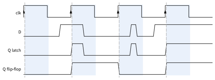
D. The latch is transparent while clk is high (shaded): its output follows D, including the short pulse, and holds its value while clk is low. The flip-flop samples D only at the rising edges (dashed) and ignores every change in between.
A flip-flop is built from two latches in series with opposite gates, the master and the slave. While the clock is low, the master is transparent and follows D, and the slave holds Q. At the rising edge, the master closes and holds the value of D at that moment, and the slave opens and passes it to Q. So the value that D has at the edge is the one that appears at Q.
Synchronous designs use flip-flops (Section 2.2.2). Their state changes only at the clock edges, so every path from one register to the next has exactly one clock period, and a tool can check each path on its own. A latch passes every change of D while it is transparent, including glitches, so a path through a latch continues into the next phase of the clock (Section 6.11). In SG13CMOS5L, the latch dlhq_1, transparent while its gate is high, has an area of 30.84 µm², and the flip-flop dfrbpq_1, which has an asynchronous reset, 48.99 µm². In synchronous designs, latches mostly appear inside cells, e.g., in the clock gate lgcp_1 (Section 7).
6.3 Timing Parameters of a Flip-Flop
A flip-flop needs time to sample D and to drive the new value to Q. The library describes this with a few parameters (Figure 33):
- The clock-to-output delay \(t_\text{cq}\) runs from the active clock edge to the change at
Q. Like the delay of a gate, it is a table over the slew of the clock and the load atQ(the arcrising_edgeof Section 5.4). - The setup time \(t_\text{su}\) is how long
Dmust be stable before the clock edge. - The hold time \(t_\text{hold}\) is how long
Dmust stay stable after the clock edge.
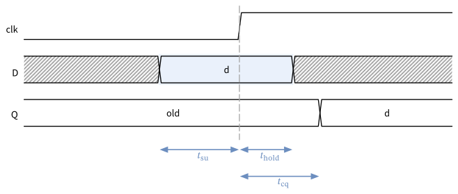
D must be stable from the setup time \(t_\text{su}\) before the edge until the hold time \(t_\text{hold}\) after it (shaded window). The new value appears at Q after the clock-to-output delay \(t_\text{cq}\). All times are measured at 50 % of the swing. The figure shows a positive hold time. A negative one ends the window before the edge.
Setup and hold time together form a window around the clock edge in which D must not change. Both are timing checks in the library, 4×4 tables over the slews of D and of the clock (Section 5.4). A hold time can be negative: then the window ends before the clock edge, and D may already change shortly before the edge. This happens when the data takes longer than the clock to reach the master latch inside the cell, so a change at D arrives there only after the master has closed.
The asynchronous reset has two checks of its own. The recovery time is how long before the clock edge RESET_B must be released, so that the flip-flop leaves the reset at this edge. The removal time is the minimum time between the clock edge and a later release, so that the flip-flop leaves the reset only at the next edge. They are the setup and hold time of the reset release. A negative removal time, as in Table 36 below, means that the release may even come shortly before the edge and still count only for the next edge. With a recovery time of 0.133 ns and a removal time of -0.114 ns, a release between 0.133 ns and 0.114 ns before the edge is forbidden. If the checks are violated, some flip-flops leave the reset one clock cycle later than others, and the design starts in a state that the RTL never reaches. Section 8 shows how a reset synchronizer prevents this. Finally, the clock and the reset need a minimum pulse width, so that the latches inside the cell can switch at all.
The script ff/ff.tcl reads these parameters of dfrbpq_1 from the tables of the library, with report_dcalc on each arc of the cell (Table 36):
cd /foss/designs/vlsi-design/content/sequential/code/ff
sta -no_init -exit ff.tclsg13cmos5l_dfrbpq_1 in the typical corner, with clock and data slews of 0.1 ns and a load of 5 fF
| Parameter | Arc | Value |
|---|---|---|
clock-to-output delay, Q rising |
CLK rising to Q rising |
0.207 ns |
clock-to-output delay, Q falling |
CLK rising to Q falling |
0.203 ns |
setup time, D rising / falling |
CLK rising to D |
0.127 / 0.121 ns |
hold time, D rising / falling |
CLK rising to D |
-0.072 / -0.043 ns |
| recovery time | CLK rising to RESET_B rising |
0.133 ns |
| removal time | CLK rising to RESET_B rising |
-0.114 ns |
| reset to output | RESET_B falling to Q falling |
0.276 ns |
minimum pulse width, CLK high / low |
CLK |
0.217 / 0.249 ns |
minimum pulse width, RESET_B low |
RESET_B |
0.233 ns |
What happens when D changes inside the window? The master latch may then capture a voltage between 0 and 1, and the flip-flop can become metastable: its output hangs at an invalid level for an unpredictable time before it settles to 0 or 1. Inside a synchronous design, the timing checks of Section 6.5 rule this out. For signals from other clock domains and for asynchronous inputs, it can happen, and Section 8 treats it.
6.4 Timing of a Register-to-Register Path
Figure 34 shows a path from FF1, which launches the data at a clock edge, to FF2, which captures it at the next edge. The clock reaches FF1 after a clock latency \(L_1\) and FF2 after a latency \(L_2\), through the buffers of the clock tree. Their difference \(t_\text{skew} = L_2 - L_1\) is the clock skew. The clock uncertainty \(t_\text{unc}\) is a margin for the jitter of the clock source, i.e., the variation of its period from cycle to cycle, and, before the clock tree exists, for its skew.
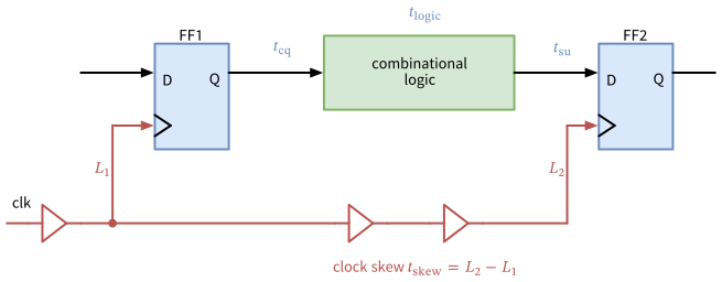
The setup condition. FF1 launches a new value at the clock edge at time 0. It appears at Q after \(t_\text{cq}\) and reaches D of FF2 after the delay \(t_\text{logic}\) of the combinational logic. FF2 captures it at the next edge, one clock period \(T\) later, and the value must arrive \(t_\text{su}\) before that edge. With the latencies, the arrival time is \(L_1 + t_\text{cq} + t_\text{logic}\), and the required time is \(T + L_2 - t_\text{su} - t_\text{unc}\). The longest path through the logic counts:
\[t_\text{cq} + t_\text{logic,max} + t_\text{su} \le T + t_\text{skew} - t_\text{unc}\]
The hold condition. The same edge at time 0 also reaches FF2, which captures the old value of FF1 there. The new value of FF1 must not arrive at FF2 before the hold window of this edge closes. Now the shortest path through the logic counts:
\[t_\text{cq} + t_\text{logic,min} \ge t_\text{hold} + t_\text{skew} + t_\text{unc}\]
The uncertainty makes both checks harder. The hold check compares the same clock edge at both registers, so the jitter of the source cancels there, and its uncertainty only needs to cover the skew. set_clock_uncertainty with -setup or -hold sets the two margins separately. The slack is the margin of a check: the required time minus the arrival time for setup, and the arrival time minus the required time for hold. A slack of zero or more means that the check is met.
Three consequences follow from the two conditions:
- The setup condition sets the clock frequency. The minimum period of a path is \(T_\text{min} = t_\text{cq} + t_\text{logic,max} + t_\text{su} - t_\text{skew} + t_\text{unc}\), and the slowest path of the design sets the maximum frequency \(f_\text{max} = 1/T_\text{min}\). With the values of Table 36, logic of 1 ns, no skew, and no uncertainty, \(T_\text{min} = 0.207 + 1 + 0.127 = 1.334\) ns.
- The hold condition does not contain the clock period. For a path between two flip-flops on the same clock edge, a hold violation fails at every clock frequency, even at a slow one. It cannot be fixed by lowering the clock frequency, and a chip with such a violation may not work at all.
- Skew helps one check and hurts the other. A capturing clock that arrives later gives the setup check more time and takes the same time away from the hold check. Hold violations therefore appear on short paths, e.g., between registers without logic in between, as in shift registers and scan chains (Section 9), when the clock reaches the capturing register late.
6.5 Static Timing Analysis
Static timing analysis (STA) checks these conditions for every path of a design, without simulating it. It splits the netlist into timing paths. A path starts at a startpoint, an input port or the clock pin of a register, and it ends at an endpoint, an output port or a data pin of a register. That gives four kinds of paths (Figure 35): from an input to a register, from register to register, from a register to an output, and from an input straight through to an output.
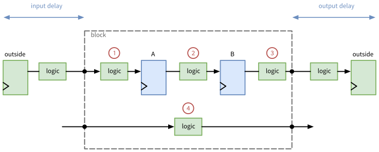
The tool builds a timing graph from the cells and nets of the netlist. Starting at the startpoints, it propagates the arrival times of a rising and of a falling transition through the graph: the latest arrival for the setup checks, the earliest for the hold checks. Each cell adds its delay, computed from its tables with the slew at its input and the load at its output (Section 5.5), and the timing sense of each arc tells which edge follows which. At every endpoint, the tool computes the required time from the capturing clock edge and the setup or hold time of the cell, and from it the slack. A design meets its timing when no slack is negative. The worst negative slack (WNS) is the smallest slack of all endpoints, the total negative slack (TNS) the sum of all negative slacks, a measure of how much work is left.
Compared with a timing simulation (Section 4.10.2), STA needs no stimuli, checks every path, and runs in a time that grows only linearly with the size of the design. It has its limits, though. STA does not know the function of the design: it also times paths that can never be activated, and it cannot tell whether a design works. And it checks exactly what the constraints describe: a clock it does not know, or a wrong input delay, gives a report full of positive slacks for a chip that fails. OpenSTA analyzes one corner per run here. Setup is usually hardest in the slow corner and hold in the fast one, but the signoff checks both in all corners (Section 5.6).
6.6 Timing Constraints
The constraints describe the clocks and the environment of a design. They are written in SDC (Synopsys Design Constraints), a set of Tcl commands that most timing and layout tools read, among them OpenSTA, OpenROAD, and LibreLane (Section 10). Here are the constraints of the barrel shifter between two registers, bs_reg:
bs_reg/syn/bs_reg.sdc
# SPDX-FileCopyrightText: 2026 Simon Dorrer
# SPDX-License-Identifier: Apache-2.0
# Description: Timing constraints of bs_reg: a 250 MHz clock, and
# inputs and outputs that connect to registers outside the block.

# The clock, ideal until the clock tree exists
create_clock -name clk -period 4.0 [get_ports clk_i]
set_clock_transition 0.1 [get_clocks clk]
set_clock_uncertainty 0.1 [get_clocks clk]

# The environment: the external registers use 1 ns of each period
set inputs [delete_from_list [all_inputs] [get_ports clk_i]]
set_input_delay 1.0 -clock clk $inputs
set_output_delay 1.0 -clock clk [all_outputs]
set_driving_cell -lib_cell sg13cmos5l_buf_2 -pin X $inputs
set_load 0.01 [all_outputs]
The clock. create_clock defines a clock with a name and a period at a port, here 4 ns, i.e., 250 MHz, with a duty cycle of 50 %. Before the layout, the clock tree does not exist yet, so the clock is ideal: it arrives at all registers at the same time, with the slew of set_clock_transition. set_clock_uncertainty adds the margin \(t_\text{unc}\) for jitter and for the skew of the future clock tree. After clock tree synthesis, set_propagated_clock makes the tool compute the real latency of every register through the buffers of the clock tree (Section 6.10).
The environment. An input of the block is driven by a register outside, which launches its data at the same clock edge. set_input_delay says how much of the period the outside path already uses, i.e., the clock-to-output delay of the external register and the logic behind it. The path from the input to the first register inside then has \(T\) minus the input delay. In the same way, set_output_delay says how much time the logic and the register behind an output need before the next clock edge. set_driving_cell tells which cell drives the inputs, so that the first cells see a realistic slew and the delay of the driver counts, and set_load sets the capacitance at the outputs. When nothing is known about the environment, a common choice is to give the inside and the outside of each port path a share of the period, as here 1 ns of 4 ns for the outside.
The timing scripts of the earlier chapters used the same commands. In Section 3.6.1, the inputs change at the clock edge and the outputs are sampled at the next edge, i.e., both delays are 0, which gives the paths through the ports the whole period. The FIFO of Section 4.10.2 gives its inputs and outputs half a period each, because its testbench changes the inputs and samples the outputs at the falling edge.
6.7 Static Timing Analysis with OpenSTA
OpenSTA (Parallax Software and The OpenROAD Project 2026) is the timing analyzer of the open-source flow, and OpenROAD and LibreLane run it internally. Synthesize bs_reg with the buffering and sizing of Section 5.7, and run its timing script:
cd /foss/designs/vlsi-design/content/sequential/code/bs_reg
yosys -p "read_verilog -sv \
  ../../../verification/code/barrel_shift/rtl/barrel_shift.sv \
  rtl/bs_reg.sv; synth -top bs_reg; flatten; \
  dfflibmap -liberty $LIB; \
  abc -constr ../../../synthesis_lib/code/synth/abc.constr \
  -liberty $LIB; opt_clean; \
  stat -liberty $LIB; write_verilog -noattr bs_reg.nl.v"
sta -no_init -exit syn/sta.tcl
bs_reg/syn/sta.tcl
# SPDX-FileCopyrightText: 2026 Simon Dorrer
# SPDX-License-Identifier: Apache-2.0
# Description: Static timing analysis of bs_reg with OpenSTA. Usage,
# in the folder bs_reg: sta -no_init -exit syn/sta.tcl (reads
# bs_reg.nl.v). CORNER selects the library corner (default
# typ_1p20V_25C).

set corner typ_1p20V_25C
if {[info exists ::env(CORNER)]} { set corner $::env(CORNER) }
set lib $::env(PDK_ROOT)/ihp-sg13cmos5l/libs.ref/sg13cmos5l_stdcell
read_liberty $lib/lib/sg13cmos5l_stdcell_$corner.lib
read_verilog bs_reg.nl.v
link_design bs_reg
read_sdc syn/bs_reg.sdc

# Missing clocks and constraints, then the worst setup and hold paths
check_setup -verbose
report_checks -path_delay max -fields {fanout} -digits 3
report_checks -path_delay min -digits 3
report_clock_min_period
report_wns -digits 3
report_tns -digits 3
report_check_types -max_slew -max_capacitance -violators
read_liberty,read_verilog, andlink_designread the library and the netlist and connect them, andread_sdcreads the constraints.check_setup -verbosereports registers without a clock and endpoints without a constraint. Run it first: a path that no constraint covers does not appear in any report.- STA sorts the endpoints into path groups, one for each capturing clock and one, called
asynchronous, for the checks of the asynchronous reset.report_checks -path_delay maxreports the path with the worst setup slack of each group,-path_delay minthe one with the worst hold slack.-fields {fanout}adds the number of pins that each net drives. report_clock_min_periodreports the minimum period of each clock from the paths between registers. With-include_port_paths, it also takes the paths from the inputs and to the outputs into account.report_wnsandreport_tnsreport the WNS and the TNS, which OpenSTA prints as 0 when no slack is negative.report_check_types -max_slew -max_capacitance -violatorslists the pins whose slew or load exceeds the limits of the library,max_transitionandmax_capacitance(Section 5.4).
The netlist has 915 cells and 15,276 µm², and check_setup finds nothing. Here is the worst setup path of the clock clk, from the flip-flop of shamt_q[1] to the one of out_q[30]:
Startpoint: _1719_ (rising edge-triggered flip-flop clocked by clk)
Endpoint: _1716_ (rising edge-triggered flip-flop clocked by clk)
Path Group: clk
Path Type: max

Fanout    Delay     Time   Description
-----------------------------------------------------------------
          0.000    0.000   clock clk (rise edge)
          0.000    0.000   clock network delay (ideal)
          0.000    0.000 ^ _1719_/CLK (sg13cmos5l_dfrbpq_1)
     1    0.204    0.204 ^ _1719_/Q (sg13cmos5l_dfrbpq_1)
     9    0.111    0.314 ^ _0812_/X (sg13cmos5l_buf_4)
    10    0.163    0.477 ^ _1279_/X (sg13cmos5l_buf_4)
    10    0.190    0.668 ^ _1556_/X (sg13cmos5l_buf_2)
    10    0.203    0.871 ^ _0906_/X (sg13cmos5l_buf_2)
     3    0.276    1.147 v _0984_/X (sg13cmos5l_mux4_1)
     2    0.132    1.279 v _1249_/X (sg13cmos5l_mux2_1)
     1    0.154    1.433 ^ _1261_/Y (sg13cmos5l_a221oi_1)
     1    0.059    1.491 v _1262_/Y (sg13cmos5l_o21ai_1)
          0.000    1.491 v _1716_/D (sg13cmos5l_dfrbpq_1)
                   1.491   data arrival time

          4.000    4.000   clock clk (rise edge)
          0.000    4.000   clock network delay (ideal)
         -0.100    3.900   clock uncertainty
          0.000    3.900   clock reconvergence pessimism
                   3.900 ^ _1716_/CLK (sg13cmos5l_dfrbpq_1)
         -0.100    3.800   library setup time
                   3.800   data required time
-----------------------------------------------------------------
                   3.800   data required time
                  -1.491   data arrival time
-----------------------------------------------------------------
                   2.308   slack (MET)
The report has two halves. The upper half follows the data: the clock edge at 0, the ideal clock network with a delay of 0, the clock-to-output delay of 0.204 ns, and then every cell of the path with its delay and the arrival time after it. ^ marks a rising, v a falling transition. This path passes four buffers, each of which drives nine or ten pins. The lower half computes the required time from the next clock edge at 4 ns, minus the uncertainty of 0.1 ns and the setup time of FF2 of 0.100 ns. The setup time is smaller than in Table 36, because the slew at D is smaller here. The difference of 2.308 ns is the slack. The clock reconvergence pessimism gives back the margin that is lost when the shared part of the launching and the capturing clock path is counted once slow and once fast. For an ideal clock, it is 0.
report_clock_min_period reports 1.69 ns, i.e., 591 MHz, for the paths between the registers: the arrival time of 1.491 ns plus the setup time and the uncertainty. The worst hold path runs from the input register data_q[0] to the output register out_q[16], with an arrival time of 0.328 ns, a required time of 0.081 ns (the uncertainty of 0.100 ns plus a hold time of -0.019 ns), and a slack of 0.247 ns.
The group asynchronous holds the recovery and removal checks of the reset. The input rst_ni drives the RESET_B pins of all 71 flip-flops through one net. The driving buf_2 needs 0.599 ns for that, and the large slew of 0.87 ns raises the recovery time to 0.323 ns. The recovery slack is still 1.977 ns. But this path limits the block: with the input delay of 1 ns, the release of the reset needs 1.0 + 0.599 + 0.323 + 0.1 = 2.022 ns, and report_clock_min_period -include_port_paths reports 2.02 ns, i.e., 494 MHz. In the layout flow, the reset net is buffered like any net with a large fanout (Section 10), and Section 8 explains how its release is made synchronous to the clock.
TipExercise: How Fast Is the Barrel Shifter?
All commands start in the folder content/sequential/code/bs_reg. The text synthesized bs_reg with the buffering and sizing of ABC. Here, you compare it with the default mapping.
- Synthesize
bs_regwith the default mapping, i.e., withabc -liberty $LIBinstead of theabc -constr ...command of the text, and runsta -no_init -exit syn/sta.tcl. How many cells does the netlist have? What are the worst negative slack, the total negative slack, and the minimum clock period? - Follow the worst setup path of the clock
clk. Where does the time go? Look up the net that the start point drives inbs_reg.nl.v, and explain what happened. What doesreport_check_typesreport? - Compute the minimum period from the report of the worst path by hand, and compare it with
report_clock_min_period. - Run the netlist of step 1 also in the slow corner:
CORNER=slow_1p08V_125C sta -no_init -exit syn/sta.tcl. Then synthesize the netlist of the text again, sincesta.tclalways readsbs_reg.nl.v, and run it in both corners. Which netlist runs at 250 MHz in both corners? What did theabc -constrcommand add to the netlist? Compare the cell lists ofstat.
Before continuing, please finish the previous exercise. Once you are done, compare with the solution below.
TipSolution: How Fast Is the Barrel Shifter?
- The default mapping gives 811 cells and 14,398 µm². The worst negative slack is -2.507 ns, the total negative slack -76.407 ns, and the minimum period 6.51 ns, i.e., 154 MHz.
- The worst path starts at
_1510_, whose outputQdrives the netshamt_q[0], the lowest bit of the registered shift amount. It drives 116 pins, and its clock-to-output delay alone is 1.971 ns. Behind it, ano21ai_1drives 35 pins (1.779 ns) and anand2_148 pins (1.758 ns): these three cells take 5.5 ns of the arrival time of 6.308 ns. Every bit of the shift amount selects in many multiplexers, and without-constr, ABC maps the logic without buffering, with the weakest cells.report_check_typesreports 208 pins whose slew, between 2.63 and 3.50 ns, exceeds the limit of 2.51 ns, and two flip-flop outputs above their maximum load of 0.30 pF:_1510_/Qwith 0.87 pF and_1511_/Qwith 0.65 pF. These delays lie beyond the tables and are extrapolated (Section 5.5). - The arrival time of 6.308 ns, plus the setup time of 0.099 ns and the uncertainty of 0.100 ns, gives 6.507 ns, which
report_clock_min_periodrounds to 6.51 ns. - In the slow corner, the minimum period is 2.58 ns for the netlist of the text and 10.14 ns for the default mapping. Only the netlist of the text runs at 250 MHz in both corners, with a setup slack of 1.42 ns between the registers in the slow corner. The default mapping misses 250 MHz even in the typical corner.
abc -constradded 104 buffers (74buf_1, 21buf_2, 8buf_4, 1buf_8), which cost 6 % more area. In Section 5.7, the purely combinational block with ideal inputs needed 3.87 ns in the slow corner with the default mapping. Driven by real flip-flops, the missing buffers make it about two and a half times slower.
6.8 Generated Clocks
A clock propagates through buffers, inverters, and gates, e.g., through a clock gate, but not through a flip-flop. When a register output clocks other registers, as slow_clk_q in the FPGA version of the LED blinker in Section 3.4.2, STA does not know this clock unless the constraints define it. create_generated_clock defines a generated clock, a clock that is derived from another one, with its source, the ratio, e.g., -divide_by 2, and the pin where it appears. The tool then knows the edges of the new clock, times the paths it clocks, and also the paths between it and its source clock, which are synchronous to each other.
TipExercise: A Clock That STA Does Not See
All commands start in the folder content/sequential/code/gen_clk. It holds the reference solution led_blink_fpga.sdc, so move it out of the way first: mv led_blink_fpga.sdc led_blink_fpga_solution.sdc.
Sketch the clock network of
led_blink_fpgaincontent/modeling/code/led_blink/exercise/led_blink_fpga.sv: which registers doesclk_iclock, and which onesslow_clk_q?Synthesize the design into this folder:
yosys -p "read_verilog -sv \
  ../../../modeling/code/led_blink/exercise/led_blink_fpga.sv; \
  synth -top led_blink_fpga; dfflibmap -liberty $LIB; \
  abc -liberty $LIB; opt_clean; \
  write_verilog -noattr led_blink_fpga.nl.v"
Write a file
clk.sdcwith a clock of 20 ns atclk_i, an output delay of 0, and a load of 10 fF atled_o. RunTOP=led_blink_fpga SDC=clk.sdc sta -no_init -exit sta.tcl. What doescheck_setupreport, and what does it mean for the analysis?Write
led_blink_fpga.sdc: add a generated clock forslow_clk_qto the constraints of step 3. Which ratio does it need? Hint: the pin of the generated clock is the output of the flip-flop that drives the netslow_clk_q, whichget_pins -of_objects [get_nets slow_clk_q] -filter "direction == output"finds. Run the analysis again. Which period doesreport_clock_propertiesshow, and which new path group appears?Synthesize the ASIC version
../../../modeling/code/led_blink/rtl/led_blink.svof Section 3.4.2 in the same way and constrain it. Which constraints does it need?
Before continuing, please finish the previous exercise. Once you are done, compare with the solution below.
TipSolution: A Clock That STA Does Not See
clk_iclocks the countercount_qand the dividerslow_clk_q, i.e., 25 flip-flops.slow_clk_qclocks onlyled_q.- Yosys maps the 26 flip-flops onto
dfrbpq_1cells with their reset tied inactive. The netlist has no initial values (Section 3.4.1). check_setupreports one unclocked register pin,_175_/CLK, the clock pin ofled_q, and two unconstrained endpoints,_175_/Dandled_o. STA does not check these paths at all: the report shows only the groupclk, and a violation behind the divider would go unnoticed.slow_clk_qtoggles everyDIV= 12,500,000 cycles, so the generated clock dividesclkby 25,000,000 (the file below).check_setupreports nothing anymore.report_clock_propertiesshowsslow_clkwith a period of 500,000,000 ns, i.e., 0.5 s, and its edges at 0 and 250,000,000 ns. The new path groupslow_clkholds the path to_175_/D. The generated clock is ideal here. In the layout, it also arrives later thanclkby the clock-to-output delay of the divider and its own clock tree (Section 3.4.2).
gen_clk/led_blink_fpga.sdc
# SPDX-FileCopyrightText: 2026 Simon Dorrer
# SPDX-License-Identifier: Apache-2.0
# Description: Timing constraints of the FPGA LED blinker of chapter
# 3: the 50 MHz clock and the clock that slow_clk_q derives from it.

create_clock -name clk -period 20 [get_ports clk_i]

# slow_clk_q toggles every DIV = 12,500,000 cycles: clk / (2 * DIV)
set div_q [get_pins -of_objects [get_nets slow_clk_q] \
  -filter "direction == output"]
create_generated_clock -name slow_clk -source [get_ports clk_i] \
  -divide_by 25000000 $div_q

set_output_delay 0 -clock clk [all_outputs]
set_load 0.01 [all_outputs]
- The ASIC version has one clock, so it needs no generated clock:
create_clockatclk_i, an input delay forrst_ni, and the output delay and the load ofled_o. Without the input delay,check_setupreportsrst_nias an input without input delay, and the reset paths are not timed. With it,check_setupreports nothing, all 26 flip-flops are in the groupclk, and theirRESET_Bpins in the groupasynchronous.
6.9 Timing Exceptions
By default, STA assumes that every path between two registers has one clock period. Timing exceptions change this for selected paths:
- A false path, set with
set_false_path, is removed from the analysis, e.g., a path from a configuration register that is written once and stays constant during operation. Paths between two unrelated clocks also need special treatment (Section 8). - A multicycle path, set with
set_multicycle_path, gets several clock periods, for logic whose result is only used every few cycles. set_max_delayandset_min_delayset a limit for a path directly, e.g., for a combinational path from an input to an output.
A multicycle path needs care. Run bs_reg with a period of 1.2 ns instead of 4 ns, and the worst setup slack between the registers becomes -0.492 ns. Suppose the RTL loads the input and the output register only every second cycle, with an enable, so that the barrel shifter has two periods. The exception for the setup check is:
set_multicycle_path 2 -setup \
  -from [all_registers] -to [all_registers]
The setup slack becomes 0.708 ns, but the hold check now fails with -0.953 ns. By default, the hold check uses the edge one period before the setup capture edge. Moving the setup edge by one period also moves the hold edge, so the new data must not reach FF2 until one period after the launch edge. The second exception moves the hold edge back to the launch edge:
set_multicycle_path 1 -hold \
  -from [all_registers] -to [all_registers]
The hold slack is back at 0.247 ns. The rule is to set -hold to one less than -setup. Every exception is a promise that the tool cannot check: if the RTL does not really wait for the second cycle, the chip fails while the timing report is clean. So keep exceptions few, and check with assertions in the RTL simulation that the design really waits (Section 4.8).
6.10 Hold Violations
Before the layout, the clock is ideal, and the uncertainty is the only margin that the hold check keeps for the skew of the future clock tree. After clock tree synthesis, set_propagated_clock makes STA compute the latency of every register through the buffers of the clock tree. A short path between two registers whose clocks arrive at different times can then fail the hold check. The layout flow repairs such paths after clock tree synthesis by inserting delay into the data path (Section 10). SG13CMOS5L has three delay cells for that, dlygate4sd1_1 to dlygate4sd3_1, with increasing delay.
A setup violation and a hold violation are fixed in opposite ways. A setup violation needs a shorter path: stronger cells, different logic, a pipeline register (Section 7), or a slower clock. A hold violation needs a longer shortest path or less skew, and the added delay must not break the setup check of the same path.
TipExercise: Fix a Hold Violation
All commands start in the folder content/sequential/code/hold. The netlist shift.v holds two flip-flops in a row, as in a shift register. The clock reaches ff1 directly and ff2 through four buf_1 cells. The script hold.tcl propagates the clock through them and reports the hold and the setup check of the path from ff1 to ff2.
- Draw the circuit with its clock path, and mark the clock edges that the hold check compares. Write the hold condition of this path with the delay of the four buffers. How large may their sum be before the check fails?
- Run the analysis in the fast, the typical, and the slow corner:
CORNER=fast_1p32V_m40C sta -no_init -exit hold.tcl, then withtyp_1p20V_25Candslow_1p08V_125C. Which corner has the worst hold slack? Explain it with the numbers of the report. - Run the slow corner with a clock period of 40 ns instead of 4 ns:
PERIOD=40 CORNER=slow_1p08V_125C sta -no_init -exit hold.tcl. What changes? - Fix the violation: copy
shift.vtoshift_orig.v, and insert asg13cmos5l_dlygate4sd1_1with the pinsAandXbetweenff1andff2. Run all three corners again. Is the hold check met everywhere, and what does the delay cell cost the setup check?
Before continuing, please finish the previous exercise. Once you are done, compare with the solution below.
TipSolution: Fix a Hold Violation
The hold check compares the launch of
ff1at a clock edge with the capture offf2at the same edge, which reachesff2later by the delay \(t_\text{buf}\) of the four buffers, the skew. The data path is only the clock-to-output delay offf1, andhold.tclsets no uncertainty, so the hold condition is \(t_\text{cq} \ge t_\text{hold} + t_\text{buf}\). The buffers may delay the clock by at most \(t_\text{cq} - t_\text{hold}\). The setup check gains the same skew and has almost the whole period.The hold slack is -0.022 ns in the fast, -0.030 ns in the typical, and -0.054 ns in the slow corner, so the slow corner is the worst. In the fast corner, the four buffers delay the clock by 0.179 ns and
ff1switches after 0.137 ns, in the slow corner after 0.388 ns and 0.288 ns. Both delays roughly double, but the skew is the larger one, so the difference grows from 0.042 to 0.100 ns. The hold time, -0.021 ns in the fast and -0.047 ns in the slow corner, makes up only part of that. The deficit consists of delays, so it grows with the delays of the corner. A hold check in the fast corner alone would have missed the worst case. With a balanced clock tree, where a fixed margin such as the uncertainty dominates, the fast corner is usually the worst.The hold slack stays at -0.054 ns, and only the setup slack grows from 3.897 ns to 39.897 ns. The clock period does not appear in the hold condition.
The netlist with the delay cell:
wire q1d;
sg13cmos5l_dlygate4sd1_1 dly (.A(q1), .X(q1d));
sg13cmos5l_dfrbpq_1 ff2 (.CLK(ck4), .D(q1d), .RESET_B(1'b1),
  .Q(q_o));
The hold check is now met in all three corners, with a slack of 0.067 ns in the fast, 0.105 ns in the typical, and 0.161 ns in the slow corner. The setup slack drops from 3.962, 3.941, and 3.897 ns to 3.881, 3.809, and 3.697 ns, i.e., by 0.08 to 0.20 ns, which a path with four nanoseconds to spare can easily afford.
6.11 Latches and Time Borrowing
A latch in a path does not cut it at a fixed time, as a flip-flop does. The netlist borrow/borrow_latch.v has a latch dllrq_1 in the middle of a path from ff1 to ff2, transparent while the clock is low. Six delay cells stand for the logic in front of it, two for the logic behind it. The latch opens at the falling edge, in the middle of the period of 4 ns, and closes at the next rising edge. Data that arrives while the latch is open passes through at once. The time that the first stage uses after the opening edge is borrowed from the second stage. In borrow/borrow_ff.v, a flip-flop on the falling edge of the clock takes the place of the latch:
cd /foss/designs/vlsi-design/content/sequential/code/borrow
TOP=borrow_ff sta -no_init -exit borrow.tcl
TOP=borrow_latch sta -no_init -exit borrow.tcl
With the flip-flop, the first stage has half a period and fails with a slack of -0.474 ns, while the second stage has 1.001 ns to spare. With the latch, OpenSTA reports that the first stage borrows 0.354 ns, and it reports a slack of 0 for the borrowing stage. The second stage starts 0.354 ns later, and the latch passes the data from D to Q a little more slowly than the flip-flop from its clock to Q, so the second stage keeps 0.620 ns of slack. The most a stage can borrow is the transparent phase minus the setup time of the latch.
Time borrowing lets latch-based designs balance their stages automatically, which is why some high-performance processors use latches. The price is a more complex timing analysis, harder hold checks, because a latch launches data already at its opening edge while the next latch holds its data until its closing edge, and a more difficult scan test (Section 9). The designs of this course use flip-flops only.
6.12 Summary
- A latch is transparent while its gate is active. A flip-flop, built from a master and a slave latch, samples its input at the clock edge. Synchronous designs use flip-flops, so that every register-to-register path has exactly one period.
- A flip-flop has a clock-to-output delay, a setup and a hold time around the clock edge, a recovery and a removal time for the release of its asynchronous reset, and minimum pulse widths. The library gives them as tables over the slews. Hold times can be negative.
- The setup condition \(t_\text{cq} + t_\text{logic,max} + t_\text{su} \le T + t_\text{skew} - t_\text{unc}\) sets the clock frequency. The hold condition \(t_\text{cq} + t_\text{logic,min} \ge t_\text{hold} + t_\text{skew} + t_\text{unc}\) does not contain the period, so for a path between flip-flops on the same edge, a lower clock frequency does not fix a hold violation.
- Static timing analysis propagates arrival times through all paths of the netlist and compares them with required times, without stimuli. It knows nothing about the function, and it checks only what the constraints describe.
- SDC constraints define the clocks with their transition and uncertainty, generated clocks, the input and output delays of the environment, the driving cells and loads, and timing exceptions.
check_setupfinds what they forgot. A multicycle path for setup needs a matching one for hold. - OpenSTA reports each path with its arrival time, required time, and slack. With its high-fanout nets buffered, the barrel shifter between two registers reaches 591 MHz between its registers in the typical corner, and the release of its reset limits the block to 494 MHz.
- Hold violations come from clock skew on short paths. Delay cells in the data path fix them, and hold must be checked in all corners.
- A latch lets a slow stage borrow time from the next one, at the price of a more complex analysis.
In Section 7, we use these reports to make a design faster, smaller, and less power-hungry: pipelining, retiming, resource sharing, and clock gating.
7 Synthesis Optimizations and Low-Power Design
In Section 5, Yosys and ABC mapped RTL onto the cells of the library, and Section 6 measured how fast the result runs. This chapter asks how a design becomes faster, smaller, and less power-hungry, and who does the work. Synthesis does part of it on its own: it picks an adder architecture, shares operators, restructures and sizes the logic, and it can even switch off clocks. The rest is the job of the designer: the architecture, the pipeline, and the decision which registers may sleep. We measure every step with the tools of the earlier chapters and add a new one, the power analysis of OpenSTA.
Note
All code of this chapter is available in the folder content/synth_opt/code of the course repository: adders between registers in adder/, two multipliers in share/, a register with an enable in clock_gate/, and the constraints and scripts that all of them use in syn/. All numbers in this chapter come from the IIC-OSIC-TOOLS image 2026.10 (Yosys 0.70, OpenSTA 3.1.0, Icarus Verilog 14.0) and the standard-cell library of SG13CMOS5L, in the typical corner unless a corner is named. The script scripts/check_synth_opt.sh reproduces all of them: run bash scripts/check_synth_opt.sh in the container from the root of the repository.
For the exercises, clone the course repository into your designs folder once, if you have not done so yet:
cd /foss/designs
git clone https://github.com/iic-jku/vlsi-design.git
In every new terminal, define the path of the typical-corner library and of the ABC constraint file of Section 5.7:
LIB=$PDK_ROOT/ihp-sg13cmos5l/libs.ref/sg13cmos5l_stdcell/lib
LIB=$LIB/sg13cmos5l_stdcell_typ_1p20V_25C.lib
CONSTR=/foss/designs/vlsi-design/content/synthesis_lib/code
CONSTR=$CONSTR/synth/abc.constr
7.1 Learning Objectives
After this chapter, you will be able to:
- tell which optimizations logic synthesis performs on the operators and on the gates, and which ones remain the job of the designer
- compare the ripple-carry adder with parallel-prefix adders, and select the adder architecture in Yosys
- explain resource sharing, and check whether synthesis has shared an operator
- shorten the critical path with a pipeline register, and explain retiming
- name the components of the power consumption of a CMOS circuit and the levers that reduce them
- estimate the power of a netlist with OpenSTA, with and without the activity of a simulation
- explain why clock gating needs an integrated clock gate, and insert one with Yosys
7.2 What Synthesis Optimizes
An optimization can act on three levels:
- The architecture. The algorithm, how many operations run in parallel, how many clock cycles a result takes, the number of pipeline stages, the memories, and the number formats are decisions of the designer. Synthesis keeps the registers of the RTL, apart from re-encoding state machines, removing unused or duplicate registers (Section 5.8), and retiming, which runs only on request (Section 7.5). A design that computes its result in one clock cycle still does so after synthesis, and a serial design stays serial. No synthesis tool turns a bubble sort into a quicksort.
- The operators. Yosys works on the operators of the RTL first. It folds constants and removes unused logic (
opt,opt_clean), extracts state machines and may re-encode them (fsm), shrinks operators to the widths that are really used (wreduce), merges identical cells (opt_merge), collects additions and multiplications into arithmetic cells (alumacc), shares operators (share,opt_share), and finally builds every operator from gates with one of the templates of its library (techmap). - The gates. ABC restructures the gates of each combinational block between the registers, maps them onto the cells of the library, and sizes and buffers them (Section 5.7). It runs twice in the commands of this course:
synthends with anabcpass that maps onto generic gates, and the commandabc -libertymaps onto the library. Only the Boolean function of the block counts, so in principle ABC may rebuild a block completely. Its algorithms work on small windows of the logic, though, and they start from the structure that Yosys hands over.
Several of these steps have switches, both in Yosys and in LibreLane, the RTL-to-GDSII flow of Section 10 (Table 37).
| Optimization | Yosys | LibreLane variable |
|---|---|---|
| adder architecture | synth -extra-map |
none |
| carry-save adder trees | always, synth -arith_tree |
SYNTH_ARITH_TREE |
| Booth multipliers | synth -booth |
SYNTH_MUL_BOOTH |
| resource sharing | share, opt_share |
always on |
| mapping, sizing, buffering | abc and its options |
SYNTH_STRATEGY |
| retiming | abc -dff |
SYNTH_ABC_DFF |
| clock gating | clockgate |
SYNTH_CLOCKGATE_MIN_WIDTH |
The synth command of Yosys runs the passes arith_tree and booth only on request, while LibreLane runs both by default. LibreLane maps with the strategy AREA 0 by default, and the counter of the AMS chip template uses DELAY 4. The following sections go through the optimizations one by one.
7.3 Adders
An adder computes for every bit \(i\) a generate \(g_i = a_i b_i\), which is 1 if the bit produces a carry by itself, and a propagate \(p_i = a_i \oplus b_i\), which is 1 if the bit passes an incoming carry on. The sum bit is \(s_i = p_i \oplus c_i\), with the carry \(c_{i+1} = g_i + p_i c_i\) into the next bit. Adders differ only in how they compute the carries.
The ripple-carry adder computes \(c_{i+1}\) from \(c_i\), one bit after the other. It is the smallest adder, one full adder per bit, but the carry passes through all \(n\) bits, so its delay grows linearly with \(n\). Written out bit by bit, it looks like this (adder/rtl/add_ripple.sv):
assign c[0] = 1'b0;
for (genvar i = 0; i < WIDTH; i++) begin : g_fa
  assign s[i]   = a_q[i] ^ b_q[i] ^ c[i];
  assign c[i+1] = (a_q[i] & b_q[i]) | (c[i] & (a_q[i] ^ b_q[i]));
end
A parallel-prefix adder combines the bits into groups. A group generates a carry if its upper part generates one, or if its upper part propagates and its lower part generates one. It propagates a carry if both parts propagate. For the generate \(G\) and the propagate \(P\) of two adjacent groups, the prefix operator \(\circ\) gives those of the combined group:
\[(G_h, P_h) \circ (G_l, P_l) = (G_h + P_h G_l,\ P_h P_l)\]
The carry out of bit \(i\) is the generate of the group of bits 0 to \(i\). Since the operator is associative, the groups can be combined in any grouping, e.g., in a tree with \(\log_2 n\) levels instead of a chain of \(n - 1\). Figure 36 compares three carry networks for 8 bits.
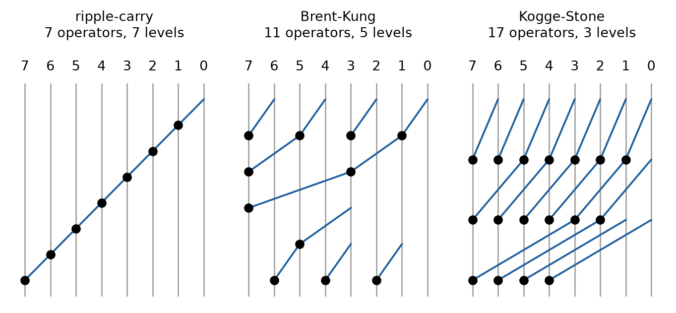
The prefix trees trade the number of operators, the wiring, and the fanout against the number of levels:
- Kogge-Stone: \(\log_2 n\) levels with \(n \log_2 n - n + 1\) operators. Every operator drives at most two others, but the network has many long wires.
- Brent-Kung: \(2 \log_2 n - 1\) levels with only \(2n - 2 - \log_2 n\) operators.
- Sklansky: \(\log_2 n\) levels with \(\frac{n}{2} \log_2 n\) operators, but the fanout doubles from level to level, up to \(n/2\) on the last level.
- Han-Carlson: Kogge-Stone on every second bit and one more level for the bits in between, i.e., \(\log_2 n + 1\) levels with fewer operators than Kogge-Stone.
For 32 bits, the ripple-carry adder has 31 operators on 31 levels, Brent-Kung 57 operators on 9 levels, and Kogge-Stone 129 operators on 5 levels. Weste and Harris treat these and further adder architectures in depth (Weste and Harris 2010).
Yosys turns + and - into an $alu cell, and techmap builds its carries with a lookahead carry unit $lcu, by default as a Brent-Kung tree (the module _90_lcu_brent_kung in techmap.v). The folder choices of Yosys holds three alternatives, which synth -extra-map selects: synth -extra-map +/choices/kogge-stone.v, and in the same way sklansky.v and han-carlson.v, where +/ stands for the data folder of Yosys. LibreLane has no switch for these prefix adders: its variable SYNTH_ADDER_TYPE only selects full-adder, ripple-carry, or carry-select adders from mapping files that the PDK must provide, and SG13CMOS5L provides none.
A sum of more than two operands, e.g., a + b + c + d, needs no chain of adders. A row of full adders adds three numbers into two, a sum and a carry vector, without passing a carry from bit to bit. A tree of such carry-save adders reduces any number of operands to two, and one final adder adds them. A multiplier works the same way: it sums its partial products, one per bit of one operand, in such a tree. Booth encoding halves the number of partial products. Yosys builds a carry-save tree for every $macc_v2 cell, i.e., for a sum of more than two operands and for the partial products of a multiplier (the pass maccmap). synth -arith_tree replaces these trees by trees of 4:2 compressors and also merges chains of separate adders, and synth -booth builds Booth multipliers.
TipExercise: Ripple or Prefix?
All commands start in the folder content/synth_opt/code/adder. The modules add_reg and add_ripple add two 32-bit numbers between an input and an output register, add_reg with + and add_ripple with the full adders written out.
Draw the prefix graphs of a 16-bit Brent-Kung and a 16-bit Kogge-Stone adder in the style of Figure 36. Count their operators and levels, and check your counts with the formulas.
Synthesize
add_ripplewith the buffering and sizing of Section 5.7, and run the timing script:cd /foss/designs/vlsi-design/content/synth_opt/code/adder yosys -p "read_verilog -sv rtl/add_ripple.sv; \ synth -top add_ripple; dfflibmap -liberty $LIB; \ abc -constr $CONSTR -liberty $LIB; opt_clean; \ stat -liberty $LIB; write_verilog -noattr add_ripple.nl.v" TOP=add_ripple sta -no_init -exit ../syn/sta.tclRepeat it for
add_regwith the default adder of Yosys and with the Kogge-Stone adder, i.e., withsynth -top add_reg -extra-map +/choices/kogge-stone.v. For each adder, note the area, the minimum period between the registers, and the number of cells on the worst path between the two flip-flops. Which adder is the fastest, and what does it cost? In each design, the 97 flip-flops take 4752 µm² of the area.Find out where the trees go. Print the longest path through the generic gates of
add_regaftersynth:yosys -p "read_verilog -sv rtl/add_reg.sv; \ synth -top add_reg; ltp -noff"Repeat it with
synth -top add_reg -noabc, which skips theabcpass at the end ofsynth. Then map all three adders without that pass and with the script../syn/keep.abc, i.e., the script ofabc -constrwithout its first steps&fraig -x,scorr,dc2, anddretime: usesynth -noabcand replaceabc -constr $CONSTRbyabc -script ../syn/keep.abc -constr $CONSTR. What do you see?Repeat step 2 with the delay-oriented ABC script
../syn/delay.abc, the strategyDELAY 4of LibreLane that the counter of the AMS chip template uses: replaceabc -constr $CONSTRbyabc -script ../syn/delay.abc -constr $CONSTR. What changes?Does the adder architecture of the RTL survive synthesis? What follows for writing arithmetic in RTL?
Before continuing, please finish the previous exercise. Once you are done, compare with the solution below.
TipSolution: Ripple or Prefix?
The Brent-Kung adder has \(2 \cdot 16 - 2 - 4 = 26\) operators on \(2 \cdot 4 - 1 = 7\) levels: 8, 4, 2, and 1 operators on the way up to bit 15, then 1, 3, and 7 on the way back down to the bits in between. The Kogge-Stone adder has \(16 \cdot 4 - 16 + 1 = 49\) operators on 4 levels: 15, 14, 12, and 8 operators, which combine each bit with the bit 1, 2, 4, and 8 positions to the right.
The results of steps 2 to 4:
Adder Mapping Cells Area (µm²) Period Cells on path ripple-carry -constr254 6462.9 4.74 ns 32 Brent-Kung -constr264 6448.4 3.83 ns 32 Kogge-Stone -constr293 6753.0 3.30 ns 27 ripple-carry keep.abc239 6372.2 4.78 ns 32 Brent-Kung keep.abc294 6809.4 2.11 ns 10 Kogge-Stone keep.abc413 7923.4 1.45 ns 7 ripple-carry delay.abc370 7580.3 2.03 ns 10 Brent-Kung delay.abc379 7741.7 2.78 ns 17 Kogge-Stone delay.abc363 7516.9 2.06 ns 12 With the mapping of Section 5.7 (step 2), the Kogge-Stone adder is the fastest, with 3.30 ns. Without the flip-flops, it needs 2001 µm², 18 % more than Brent-Kung with 1696 µm². The ripple-carry adder needs about the same area as Brent-Kung and is 24 % slower. Its worst path passes a
nand2_2and then 31 alternatinga21oi_2ando21ai_1cells, one per bit, i.e., the carry chain \(c_{i+1} = g_i + p_i c_i\) in inverting form. The worst paths of the prefix adders pass 32 and 27 cells, many more than the levels of their trees.After
synth -noabc, the longest path ofadd_regpasses 18 generic gates, aftersynth62, almost as many as the 63 of the ripple-carry adder (Kogge-Stone: 11 and 42). Theabcpass at the end ofsynthflattens the trees: its default script containsdc2, which rewrites the logic for fewer gates and does not keep its depth. The script ofabc -constrruns the same steps again, sosynth -noabcalone does not help: withabc -constr, the prefix adders still need 3.73 and 3.45 ns. Without these steps, the trees survive, and the textbook order appears: ripple-carry 4.78 ns with 32 cells on its path, Brent-Kung 2.11 ns with 10, and Kogge-Stone 1.45 ns with 7. Kogge-Stone is now 3.3 times as fast as the ripple-carry adder, and its logic twice as large (3172 against 1620 µm²).With the delay-oriented script, all three adders become faster and larger than with
-constr. The ripple-carry adder is now about as fast as Kogge-Stone (2.03 against 2.06 ns), with 10 cells on its worst path, among them wide gates such asnor4_1andor4_1, and Brent-Kung is now the slowest. The script collapses the carry chain into a few levels of wide gates. The adder logic grows by 38 to 76 %, e.g., from 1711 to 2828 µm² for the ripple-carry adder. The result depends on the starting point, though: from the netlists ofsynth -noabc, the same script gives 2.21, 1.86, and 2.00 ns.Only if no step throws it away. The default scripts of ABC rewrite the logic for area and flatten the prefix trees. A script that keeps the structure keeps the architecture and gives the fastest adder of all, and a delay-oriented script rebuilds the arithmetic in a way that depends on where it starts. So write arithmetic with its operators,
+instead of full adders, select the architecture and the script with the options of the tools, and compare the results with STA. In this flow, ABC never moves logic across a register: it only sees the logic between the flip-flops (Section 7.5). For more speed than the best mapping gives, the adder needs a pipeline.
7.5 Pipelining and Retiming
The setup condition of Section 6.4 gives a register-to-register path the minimum period \(T_\text{min} = t_\text{cq} + t_\text{logic,max} + t_\text{su} - t_\text{skew} + t_\text{unc}\). ABC can only shorten the logic between the registers. A pipeline register splits the logic into stages, each of which has a full clock period (Figure 37 (a)). With \(k\) stages of equal delay,
\[T_\text{min} = t_\text{cq} + \frac{t_\text{logic,max}}{k} + t_\text{su} - t_\text{skew} + t_\text{unc}.\]
The pipeline delivers one result per clock cycle at a higher clock frequency, i.e., a higher throughput, but every result appears \(k - 1\) cycles later than without the pipeline, i.e., the latency grows. The price is the pipeline registers, their area and their clock power (Section 7.6). The overhead \(t_\text{cq} + t_\text{su} + t_\text{unc}\) of each stage limits the gain: with the values of Table 36 and an uncertainty of 0.1 ns, no stage can be clocked with a period below about 0.43 ns.
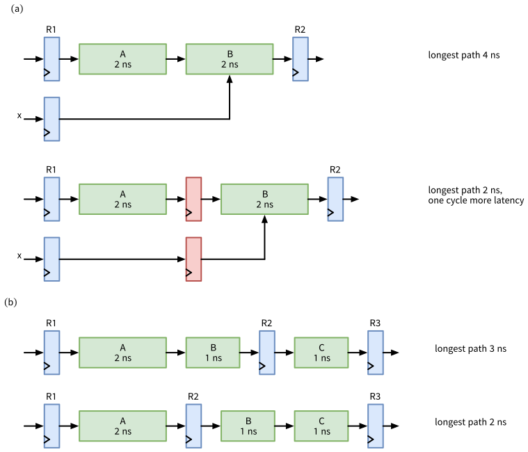
x, which enters the second half, needs a pipeline register as well. The result appears one clock cycle later. (b) Retiming: the register R2 moves backwards across the logic block B, and the longest path shrinks from 3 to 2 ns, while the function at the outputs stays the same. The delays are examples, without the clock-to-output delay and the setup time.
The work of pipelining is in the details. Every signal that belongs to the same operation must pass the same number of registers, also an operand that is only used in a later stage, such as x in the figure, and the control signals that travel along, such as a valid flag. Every testbench and every block that uses the result must expect it later.
Retiming moves registers across combinational logic without changing the behavior at the outputs (Figure 37 (b)), e.g., to balance the stages of a pipeline that is cut at the wrong place. Retiming can change the number of registers, it must compute new reset or initial values for the registers it moves, and it breaks the matching of the registers by name in equivalence checking (Section 5.8). Commercial synthesis tools retime on request. In the open-source flow, Yosys passes flip-flops to ABC only with abc -dff (in LibreLane SYNTH_ABC_DFF, off by default), and only flip-flops without a reset: yosys -h abc lists $_DFF_?_ and $_DFFE_??_. Every default script of ABC then runs dretime, which by default retimes for minimum area, i.e., it moves registers to reduce their number, not the delay. Only with a delay target, abc -dff -D <ps>, does ABC add a delay-oriented retime. And abc -dff must run before dfflibmap, while the flip-flops are still generic cells. The designs of this course use flip-flops with an asynchronous reset and place their pipeline registers in the RTL.
TipExercise: Pipeline the Adder
All commands start in the folder content/synth_opt/code/adder. It holds the reference solution rtl/add_pipe.sv, so move it out of the way first: cd /foss/designs/vlsi-design/content/synth_opt/code/adder, then mv rtl/add_pipe.sv add_pipe_solution.sv.
Draw
add_regas a pipeline with two stages: the first stage adds the lower 16 bits of the operands, the second stage the upper 16 bits with the carry of the first stage. Which signals need a pipeline register between the stages? How many flip-flops does the design have in total?Write
rtl/add_pipe.svwith the ports ofadd_reg. Check it withverilator --lint-only -Wall rtl/add_pipe.sv, and simulate it with the testbench:iverilog -g2012 -o sim.vvp rtl/add_pipe.sv tb/tb_add_pipe.sv vvp -n sim.vvpThe testbench applies new random operands in every clock cycle and expects each sum three clock edges later. Its first operands,
32'hffffffffand 1, need the carry from the first into the second stage.Synthesize
add_pipewith the commands of the previous exercise, i.e., withabc -constr $CONSTR, and runTOP=add_pipe sta -no_init -exit ../syn/sta.tcl. Compare the cells, the area, the flip-flops, and the minimum period between the registers withadd_reg. Estimate the period ofadd_pipefrom the one ofadd_regwith the formula for \(k\) stages and the overhead of 0.43 ns, and compare it with the measured period. Where is the worst path, and what explains the difference?report_clock_min_period -include_port_pathsreports a longer period foradd_pipe, but not foradd_reg. Which path sets it, and why does it matter only after pipelining? Hint: copy../syn/sta.tclto../syn/all.tcl, so that it still findsblock.sdc, and replace itsreport_checkscommand byreport_checks -path_delay max -fields {fanout} -digits 3, which reports the worst path of every path group, and runTOP=add_pipe sta -no_init -exit ../syn/all.tcl.
Before continuing, please finish the previous exercise. Once you are done, compare with the solution below.
TipSolution: Pipeline the Adder
- Between the stages, the lower sum with its carry (17 bits) and the upper halves of both operands (2 × 16 bits) need a pipeline register, 49 flip-flops in addition to the 97 of
add_reg, 146 in total. The upper halves wait one cycle, so that they meet the carry of their own lower halves. The lower sum waits for the upper sum in the pipeline register. - The module of the reference solution:
adder/rtl/add_pipe.sv
// SPDX-FileCopyrightText: 2026 Simon Dorrer
// SPDX-License-Identifier: Apache-2.0
// Description: The adder of add_reg in two pipeline stages. Stage 1
// adds the lower halves, stage 2 the upper halves with the carry of
// stage 1. The sum appears one clock cycle later than in add_reg.

`default_nettype none

module add_pipe #(
  parameter int unsigned WIDTH = 32  // even
) (
  input  logic             clk_i,
  input  logic             rst_ni,
  input  logic [WIDTH-1:0] a_i,
  input  logic [WIDTH-1:0] b_i,
  output logic [WIDTH:0]   sum_o
);

  localparam int unsigned H = WIDTH / 2;

  logic [WIDTH-1:0] a_q, b_q;
  logic [H:0]       lo_q;            // lower sum and its carry
  logic [H-1:0]     a_hi_q, b_hi_q;  // upper halves, one stage later
  logic [H:0]       hi;

  // Register process: input register, pipeline register, output
  always_ff @(posedge clk_i or negedge rst_ni) begin
    if (!rst_ni) begin
      a_q    <= '0;
      b_q    <= '0;
      lo_q   <= '0;
      a_hi_q <= '0;
      b_hi_q <= '0;
      sum_o  <= '0;
    end else begin
      a_q    <= a_i;
      b_q    <= b_i;
      lo_q   <= a_q[H-1:0] + b_q[H-1:0];
      a_hi_q <= a_q[WIDTH-1:H];
      b_hi_q <= b_q[WIDTH-1:H];
      sum_o  <= {hi, lo_q[H-1:0]};
    end
  end

  // Stage 2: the upper halves and the carry of the lower half
  assign hi = a_hi_q + b_hi_q + lo_q[H];

endmodule

`default_nettype wire
The testbench prints 1000 sums, 0 errors. Without the carry lo_q[H] in the sum of the upper halves, it reports 489 errors. The width of hi matters: as the target of an assignment, the 17-bit hi makes the addition 17 bits wide, so its carry is kept. Inside a concatenation such as {a_hi_q + b_hi_q + lo_q[H], lo_q[H-1:0]}, the sum would only be 16 bits wide.
add_pipehas 303 cells, 8852 µm², and 146 flip-flops, against 264 cells, 6448 µm², and 97 flip-flops ofadd_reg. Its minimum period is 2.34 ns (427 MHz) instead of 3.83 ns (261 MHz), i.e., it is 1.6 times faster for 37 % more area. The formula predicts \((3.83 - 0.43)/2 + 0.43 = 2.13\) ns. The worst path ends atlo_q[16], the carry out of the first stage, after 17 cells and 2.127 ns, while the 32-bit adder ofadd_regneeds 32 cells and 3.629 ns. The second stage ends after 2.102 ns, so both stages are about equally long. But each half of the adder needs more than half of the logic delay of the whole adder: 1.90 ns instead of 1.70 ns.- With the port paths,
add_pipeneeds 2.78 ns. The path is the release of the reset: the driving cellbuf_2ofblock.sdcneeds 1.225 ns to drive the 146RESET_Bpins ofrst_ni, and the large slew raises the recovery time to 0.458 ns. With the input delay of 1 ns and the uncertainty, this adds up to 2.78 ns. Inadd_reg, the same path needs only about 2.3 ns, less than the 3.83 ns between the registers, so it does not show. Pipelining shortened the paths between the registers below the reset path and added 49 loads to the reset net. In the layout flow, the reset net gets a buffer tree (Section 6.7, Section 10).
7.6 Power Consumption
A CMOS circuit consumes power in three ways:
- Switching power. A transition from 0 to 1 at a net charges its capacitance \(C\), i.e., the inputs of the cells that the net drives and its wire, from the supply, and a transition from 1 to 0 discharges it to ground. On average, each transition dissipates \(\frac{1}{2} C V^2\). With the activity \(a\), the average number of transitions per clock cycle, a net dissipates \(P_\text{sw} = \frac{1}{2} a C V^2 f\) at the supply voltage \(V\) and the clock frequency \(f\). The clock toggles twice per cycle, \(a = 2\), more than any data net without glitches.
- Internal power. Inside a cell, internal nodes switch as well, and during an edge, the pull-up and the pull-down network both conduct for a short time. The Liberty file gives the energy of each transition at a pin, the
internal_powerof Section 5.4: for an output as a table over the slew and the load, for an input over the slew, often depending on the state of the other pins. A flip-flop consumes internal power at every clock edge, even when its value does not change, because the clock switches its internal inverters and latches. - Leakage power. A transistor that is off still conducts a small current. The Liberty file gives the leakage of each cell,
cell_leakage_power, and the leakage per input state (Section 5.4). Leakage flows as long as the supply is on, whatever the circuit does.
Switching and internal power together form the dynamic power, the leakage is the static power. The levers follow from the formula:
- The supply voltage enters squared, but at a lower voltage, the cells are slower.
- The clock frequency enters linearly. The energy per operation stays the same, though: a slower clock lowers the power, but not the energy of a computation. It saves energy only together with a lower supply voltage, which the longer period allows.
- The activity drops when the clock of idle registers is switched off (clock gating, Section 7.7), when the operands of an unused operator are held constant (operand isolation), and when there are fewer glitches, the short pulses that unequal path delays produce at the output of a gate before it settles.
- The capacitance drops with smaller cells, shorter wires, and fewer buffers, so area and power go together.
- The leakage of an idle block disappears when switches cut off its supply (power gating). This needs isolation cells at the outputs of the block, a way to keep or restore its state, and a power-aware flow, which goes beyond this course. Libraries of advanced technologies also offer each cell with several threshold voltages, so that a path with slack can use slower cells that leak less.
7.6.1 Power Analysis with OpenSTA
OpenSTA computes the power of a netlist from the Liberty file, i.e., the pin capacitances, the internal power tables, and the leakage, and from the activity of every net. Without a simulation, it assumes by default that every input toggles in 10 % of the clock cycles, i.e., with an activity of 0.1 and a duty of 0.5, i.e., the input is 1 half of the time, and it propagates these activities through the logic. With a VCD file from a simulation of the netlist, read_vcd annotates the real activity of every net instead. The script syn/power.tcl does both:
syn/power.tcl
# SPDX-FileCopyrightText: 2026 Simon Dorrer
# SPDX-License-Identifier: Apache-2.0
# Description: Power analysis of a netlist <TOP>.nl.v in the current
# folder with OpenSTA and the constraints block.sdc. Usage:
# TOP=cg_reg sta -no_init -exit ../syn/power.tcl. VCD names a file
# with the activity of a simulation, whose testbench tb_<TOP> has
# the instance dut. Without VCD, every input except rst_ni toggles
# in 10 % of the clock cycles.
# CORNER selects the library corner (default typ_1p20V_25C).

set top $::env(TOP)
set corner typ_1p20V_25C
if {[info exists ::env(CORNER)]} { set corner $::env(CORNER) }
set lib $::env(PDK_ROOT)/ihp-sg13cmos5l/libs.ref/sg13cmos5l_stdcell
read_liberty $lib/lib/sg13cmos5l_stdcell_$corner.lib
read_verilog $top.nl.v
link_design $top
read_sdc [file dirname [info script]]/block.sdc

# The activity of every net: from the simulation if there is one,
# otherwise the default activity at the inputs and a quiet reset
if {[info exists ::env(VCD)]} {
  read_vcd -scope tb_$top/dut $::env(VCD)
  report_activity_annotation
} else {
  set_power_activity -input_ports rst_ni -activity 0 -duty 1
}
report_power -digits 3
Without a simulation, the script keeps the reset inactive, since a reset that toggles in every tenth cycle would not be realistic. Here is the barrel shifter between two registers of Section 6.7, synthesized with the commands of that section:
cd /foss/designs/vlsi-design/content/sequential/code/bs_reg
TOP=bs_reg sta -no_init -exit ../../../synth_opt/code/syn/power.tcl
report_power sorts the cells into groups (Table 38): the flip-flops into Sequential, the logic into Combinational, the cells of the clock network, such as clock buffers and clock gates, into Clock, and the macros and pads into groups of their own, which are empty here. The switching power of a net counts for the cell that drives it.
bs_reg at 1.2 V and 250 MHz in the typical corner, with the default activity of 0.1 at its inputs
| Group | Internal | Switching | Leakage | Total |
|---|---|---|---|---|
Sequential (71 flip-flops) |
1.126 mW | 0.030 mW | 0.04 µW | 1.156 mW |
Combinational |
0.329 mW | 0.234 mW | 0.15 µW | 0.563 mW |
Total |
1.455 mW | 0.264 mW | 0.19 µW | 1.719 mW |
The block consumes 1.72 mW, and 67 % of it in the flip-flops, 16.3 µW in each of them, although its inputs change in only one of ten cycles: the clock reaches every flip-flop in every cycle. Internal power dominates, and leakage is negligible at 25 °C. The group Clock is empty, because the netlist has no clock buffers before the layout, so a power analysis before clock tree synthesis misses the power of the clock tree.
The library of SG13CMOS5L is also characterized at 1.5 V. With CORNER=typ_1p50V_25C, the same netlist consumes 2.78 mW, 1.62 times as much, close to \((1.5/1.2)^2 = 1.56\), and the leakage rises from 0.19 to 0.56 µW. In return, the timing script of Section 6.7 reports a minimum period of 1.17 ns instead of 1.69 ns with CORNER=typ_1p50V_25C sta -no_init -exit syn/sta.tcl. The supply voltage trades speed against power.
7.7 Clock Gating
A register that keeps its value most of the time still consumes clock power in every cycle. SG13CMOS5L has no flip-flop with an enable (Section 3.4.3), so synthesis builds a register with an enable from a multiplexer in front of each flip-flop, which feeds back Q while the enable is low (Figure 38 (a)). Clock gating switches off the clock of the whole register instead, with one gate for all its flip-flops and without multiplexers (Figure 38 (b)).
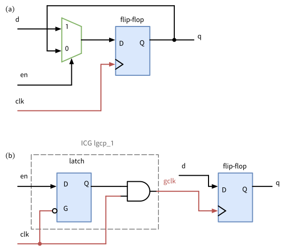
Q while en is low, and the flip-flop is clocked in every cycle. (b) An integrated clock gate (ICG), here sg13cmos5l_lgcp_1, switches off the clock of the whole register while en is low. Its latch is transparent while clk is low, so a change of en reaches the AND gate only while clk is low, and gclk has only complete pulses.
A plain AND gate of clock and enable does not work (Figure 39). The enable comes from a register on the same clock, so it changes shortly after the rising edge, while the clock is high, and the AND gate passes the change at once. A rising enable produces a late clock edge, a falling one a short pulse, which clocks the register at the wrong time or violates the minimum pulse width of its flip-flops (Section 6.3).
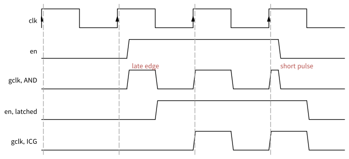
en comes from a register on the same clock, so it changes shortly after the rising edges (dashed), while clk is high. The AND gate passes these changes to its output: a late edge in the second period and a short pulse in the fourth. The latch of the ICG passes en only while clk is low, so the gated clock has only complete pulses, at the third and the fourth edge.
An integrated clock gate (ICG) puts a latch, transparent while the clock is low, in front of the AND gate. The enable reaches the AND gate only during the low phase and stays stable while the clock is high, so the gated clock has only complete pulses. A flip-flop on the falling edge in place of the latch would give clean pulses as well, but the enable would have to arrive by the falling edge, i.e., within half a period. The latch accepts it until the rising edge. In SG13CMOS5L, the ICG is lgcp_1 with the pins GATE, CLK, and GCLK and an area of 27.2 µm², and its Liberty file marks it with clock_gating_integrated_cell : "latch_posedge". Its sibling slgcp_1 has an additional input SCE, which switches the clock on during the scan test (Section 9).
The clock passes through the ICG from CLK to GCLK, so STA times the gated flip-flops with the clock of the ICG. The path of the enable ends at the pin GATE, where the library defines a clock gating check, a setup and a hold check against the rising edge of CLK. Like the data input of a flip-flop, the enable must be stable shortly before the rising edge. The ICG also delays the clock of the gated flip-flops, which clock tree synthesis balances against the other flip-flops (Section 10).
Yosys inserts the ICGs with the pass clockgate, between synth and dfflibmap. It replaces each group of flip-flops that share a clock and an enable by one ICG and flip-flops without enable:
clockgate -pos sg13cmos5l_lgcp_1 GATE:CLK:GCLK -min_net_size 4-pos names the ICG for flip-flops on the rising edge and its pins for the enable, the clock, and the gated clock. -min_net_size sets the smallest group that gets an ICG, since an ICG is clocked in every cycle and costs area and power of its own. LibreLane runs the same pass when SYNTH_CLOCKGATE_MIN_WIDTH is set, and it inserts ICGs when SYNTH_CLOCKGATE_POSEDGE_ICG names the cell, e.g., sg13cmos5l_lgcp_1/GATE/CLK/GCLK. The configuration of SG13CMOS5L sets neither and even excludes lgcp_1 and slgcp_1 from synthesis, so LibreLane gates no clocks unless a design configures it.
TipExercise: Gate the Clock
All commands start in the folder content/synth_opt/code/clock_gate. The module rtl/cg_reg.sv is a 32-bit register with the enable en_i. The testbench tb/tb_cg_reg.sv simulates its netlist for 1600 clock cycles at 250 MHz, applies new random data in every cycle, sets en_i high in one of EVERY cycles (default 16), compares the output with a model, and writes the activity of every net into cg_reg.vcd.
Draw
clk,en_i, the latched enable, andGCLKof the ICG in the style of Figure 39, for an enable that a flip-flop onclksets high for exactly one cycle. At which rising edge do the gated flip-flops loaddata_i, and is it the same edge as in the version with multiplexers?Synthesize
cg_regwithout clock gating:cd /foss/designs/vlsi-design/content/synth_opt/code/clock_gate yosys -p "read_verilog -sv rtl/cg_reg.sv; synth -top cg_reg; \ dfflibmap -liberty $LIB; abc -constr $CONSTR -liberty $LIB; \ opt_clean; stat -liberty $LIB; write_verilog -noattr cg_reg.nl.v"Which cells does the netlist have? Simulate the netlist with the models of the cells, and run the power analysis with the activity of the simulation:
CELLS=$PDK_ROOT/ihp-sg13cmos5l/libs.ref/sg13cmos5l_stdcell/verilog
iverilog -g2012 -gno-specify -o sim.vvp $CELLS/sg13cmos5l_udp.v \
  $CELLS/sg13cmos5l_stdcell.v cg_reg.nl.v tb/tb_cg_reg.sv
vvp -n sim.vvp
TOP=cg_reg VCD=cg_reg.vcd sta -no_init -exit ../syn/power.tcl
Icarus Verilog prints the 68
sorrymessages of Section 4.10.2, which do not matter without delays. How much power does the register consume? Is the share of the flip-flops larger or smaller than inbs_reg, and why? Which cells besides the flip-flops and the multiplexers does the netlist have, and why?Insert
clockgate -pos sg13cmos5l_lgcp_1 GATE:CLK:GCLK -min_net_size 4;aftersynth -top cg_reg;and repeat step 2. Compare the cells, the area, and the power. What consumes the power that remains?Repeat steps 2 and 3 with the enable high in every cycle, i.e., with
-P tb_cg_reg.EVERY=1added to theiverilogcommand. Compare again. Which entry of the reports makes the comparison unfair, and by how much?
Before continuing, please finish the previous exercise. Once you are done, compare with the solution below.
TipSolution: Gate the Clock
- The flip-flop sets
en_ishortly after a rising edge, call it edge 1, and clears it shortly after edge 2. The latch passes the high enable during the low phase after edge 1 and holds it whileclkis high after edge 2, soGCLKhas exactly one complete pulse, at edge 2. During the low phase after edge 2, the latch passes the low enable, and the pulse at edge 3 is suppressed. The gated flip-flops loaddata_iat edge 2, the same edge at which the version with multiplexers loads it, since its flip-flops sampleen_i= 1 at edge 2. - The netlist has 67 cells and 2223 µm²: 32
dfrbpq_1, 32 multiplexers (30mux2_1, 2mux2_2), and 3buf_8, which drive the enable to the 32 select inputs. The simulation reports1600 cycles, en_i in 1 of 16, 0 errors, and OpenSTA annotates the activity of all 329 pins. The register consumes 490 µW, 474 µW of it in the flip-flops (97 %, almost all internal power) and 16 µW in the multiplexers and buffers. The share of the flip-flops is larger than the 67 % inbs_reg, because the register has no logic besides the multiplexers. It changes in only one of 16 cycles, but its flip-flops are clocked in every cycle. - With
clockgate, the netlist has 33 cells and 1595 µm², 28 % less: 32dfrbpq_1and onelgcp_1, and no multiplexers. The simulation passes again. The power drops to 89.6 µW, 82 % less: 82.5 µW in the flip-flops and 7.1 µW in the groupClock, i.e., 4.8 µW of internal power in the ICG and 2.3 µW for switching the gated clock net. Of the power in the flip-flops, the clock edges in one of 16 cycles cause only a part. Without the multiplexers, the new random data reaches theDpins in every cycle, which costs internal power in the flip-flops even without a clock edge: the Liberty file gives the pinDofdfrbpq_1an internal power of its own. With data that changes only together with the enable, i.e., withdata = $urandomonly in the cycles in which the testbench setsen, the flip-flops of the gated register consume 39.6 µW. - With the enable high in every cycle, the register without clock gating consumes 673 µW (631 µW in the flip-flops, 41 µW in the multiplexers), and the one with clock gating 665 µW (621 µW in the flip-flops, 43.9 µW in the group
Clock). The groupClockof the gated register includes 36.4 µW for switching the gated clock net with its 32 clock pins. The register without clock gating has the same net, but its driver is the input portclk_i, which belongs to no cell, so OpenSTA charges its power nowhere. The gated register has such a net as well, fromclk_ito the pinCLKof the ICG, but with its 4.9 fF, it costs only about 1.8 µW. Compared fairly, the register without clock gating needs about 709 µW and the one with clock gating about 667 µW, so the ICG still saves about 6 %, because it replaces the multiplexers. With the enable in one of 16 cycles, the fair comparison is 527 µW against 91 µW. For a register of a few bits, however, an ICG that is clocked in every cycle may cost more than it saves, which is what-min_net_sizeis for.
7.8 Summary
- Synthesis optimizes the operators (Yosys) and the gates (ABC) of a design, but not its architecture: it keeps the latency and the algorithm of the RTL, and, apart from retiming on request, its registers. Pipelines, parallelism, and the choice of the algorithm remain the job of the designer.
- A ripple-carry adder is small and slow, a parallel-prefix adder computes the carries in a tree of \(\log_2 n\) to \(2 \log_2 n - 1\) levels. Yosys builds a Brent-Kung adder by default and others on request. The default scripts of ABC rewrite for area and flatten the prefix trees. A script that keeps the structure keeps the architecture, and a delay-oriented script restructures even a ripple-carry adder into a few levels of wide gates, at the price of area.
- Operations that are never needed in the same cycle can share an operator. Yosys 0.70 shares multipliers only without
alumacc, so write the sharing into the RTL where it matters, and check the result withstat. - A pipeline register shortens the critical path and raises the throughput, at the cost of latency, registers, and a fixed overhead per stage. Retiming moves registers across logic, but in the open-source flow only flip-flops without reset.
- CMOS circuits consume switching, internal, and leakage power. Dynamic power grows with \(a C V^2 f\), so the supply voltage is the strongest lever, and the activity the one that the design controls. In synchronous designs, the flip-flops and the clock take a large share, and a power analysis before clock tree synthesis does not see the clock tree.
- OpenSTA estimates power from the Liberty file and the activity of every net, which comes from a default assumption or from the VCD file of a simulation.
- Clock gating switches off the clock of idle registers. It needs an integrated clock gate whose latch keeps the enable stable while the clock is high. Yosys inserts it with
clockgate, and on a 32-bit register with an enable in one of 16 cycles, it saves more than 80 % of the power and 28 % of the area.
In Section 8, the designs get more than one clock, and we see how signals cross safely from one clock domain to another.
8 Clock Domains, Metastability, and Resets
So far, every design of this course has run on one clock or on a clock derived from it, and static timing analysis checked every path from one register to the next. Real chips have several clocks: a processor clock, the clock of an SPI master outside the chip, 48 MHz for USB, 32.768 kHz for a real-time clock, the sample clock of an ADC. And many input pins are driven by a world that knows nothing about our clock. Wherever a signal crosses from one clock to another, the capturing flip-flop sees its data change at an arbitrary moment, and sooner or later inside its setup and hold window. This chapter measures what happens then, shows how synchronizers make it rare enough, how buses and data streams cross safely, how STA must be told about crossings, and how a reset is released safely.
Note
All code of this chapter is available in the folder content/cdc/code of the course repository: the metastability measurement in meta/, the synchronizers and their simulation model in sync/, a counter that crosses two clock domains in gray/, the asynchronous FIFO in fifo/, and the reset synchronizer in reset/. All numbers in this chapter come from the IIC-OSIC-TOOLS image 2026.10 (ngspice 47, Yosys 0.70, OpenSTA 3.1.0, Icarus Verilog 14.0) and SG13CMOS5L, in the typical corner unless a corner is named. The script scripts/check_cdc.sh reproduces all of them: run bash scripts/check_cdc.sh in the container from the root of the repository.
For the exercises, clone the course repository into your designs folder once, if you have not done so yet:
cd /foss/designs
git clone https://github.com/iic-jku/vlsi-design.git
In every new terminal, define the path of the typical-corner library and of the ABC constraint file of Section 5.7:
LIB=$PDK_ROOT/ihp-sg13cmos5l/libs.ref/sg13cmos5l_stdcell/lib
LIB=$LIB/sg13cmos5l_stdcell_typ_1p20V_25C.lib
CONSTR=/foss/designs/vlsi-design/content/synthesis_lib/code
CONSTR=$CONSTR/synth/abc.constr
8.1 Learning Objectives
After this chapter, you will be able to:
- tell synchronous from asynchronous clocks, and find the clock domain crossings of a design
- explain metastability, measure the time constant of a flip-flop, and compute the mean time between failures of a synchronizer
- synchronize a level and a pulse into another clock domain
- explain why a bus whose bits can change at the same time cannot cross through one synchronizer per bit, and cross it with Gray code, a handshake, or an asynchronous FIFO
- simulate clock domain crossings with metastability injection
- constrain clock domain crossings in SDC
- release an asynchronous reset synchronously with a reset synchronizer
8.2 Clock Domains
A clock domain is the set of registers that one clock drives. Two clocks are synchronous if they come from the same source with a known phase relation, e.g., a clock and the clock divided from it by a counter. Once the constraints define the derived clock with create_generated_clock, STA knows their edges and times the paths between them like any other path (Section 6.8). Two clocks are asynchronous if they come from different sources, e.g., two crystal oscillators, or if their phase relation is unknown. Their phase drifts, so a signal from domain A reaches the registers of domain B at an arbitrary moment relative to clk_b. An asynchronous input from a pin is a crossing as well: a button, a sensor, or a chip outside on its own clock runs in a domain of its own. An input that comes from a register on the same clock, as in the constraints of Section 6.6, is timed with set_input_delay instead.
A clock domain crossing (CDC) is a path that starts at a register of one domain and ends at a register of another. Inside a synchronous design, the setup and hold checks of Section 6.5 guarantee that no flip-flop ever sees its data change inside its window. At a crossing between asynchronous clocks, no check can guarantee that, and every crossing violates the window from time to time.
8.3 Metastability
The master latch of a flip-flop (Section 6.2) stores its value in two cross-coupled inverters. This loop has two stable states, 0 and 1, and an unstable balance point in between, like a ball on the top of a hill. If D changes just at the moment the master closes, the loop starts close to the balance point, and the flip-flop is metastable. The small voltage difference grows exponentially, with a time constant \(\tau\) of the loop, until the loop reaches 0 or 1. The closer the data edge was to the critical moment, the smaller the start difference and the longer it takes. Meanwhile, the output may show a voltage between 0 and 1 or switch late, and two flip-flops behind it may see different values.
The script meta/dff_meta.py measures this with ngspice on the transistor netlist of dfrbpq_1 from the PDK (libs.ref/sg13cmos5l_stdcell/spice/sg13cmos5l_stdcell.spice), with a load of 5 fF and edges of 0.15 ns. It moves a rising D toward the rising clock edge and finds, by bisection to \(10^{-19}\) s, the latest arrival that the flip-flop still captures. Then it moves the data edge away from that critical point by \(\delta\), decade by decade, and measures the clock-to-output delay. The netlist of the PDK is the schematic of the cell, without the wiring capacitance of its layout, so the script adds an estimated 1.5 fF to each of its 15 internal nodes:
cd /foss/designs/vlsi-design/content/cdc/code/meta
python3 dff_meta.py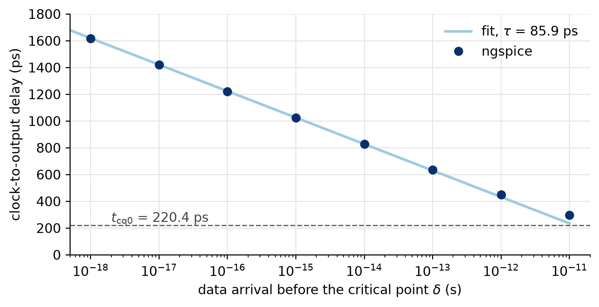
sg13cmos5l_dfrbpq_1 in ngspice, typical corner, with 1.5 fF at each internal node, over the time \(\delta\) by which the rising D arrives before the latest arrival that the flip-flop still captures. Every decade closer to that point adds about 198 ps, i.e., \(\tau \ln 10\) with \(\tau\) = 85.9 ps. Far from the point, the delay approaches its normal value \(t_\text{cq0}\) = 220.4 ps. The line is the fit from \(10^{-17}\) to \(10^{-14}\) s.
Figure 40 shows the result. Without metastability, the clock-to-output delay is \(t_\text{cq0}\) = 220.4 ps. Near the critical point, every decade adds about 198 ps. The delay follows
\[t_\text{cq} = t_\text{cq0} + \tau \ln \frac{T_0}{2\delta},\]
with \(\tau\) = 85.9 ps and \(T_0\) = 23.5 ps from a fit from \(10^{-17}\) to \(10^{-14}\) s. Farther from the point, the start difference of the latch is no longer small, and the delay approaches its normal value. How good is the estimate of the wiring capacitance? The library gives a clock-to-output delay of 0.202 ns for the same edges, whose slew from 20 to 80 % is 0.09 ns, and the same load, a little less than the 0.207 ns of Table 36 at slews of 0.1 ns. With the estimate, \(t_\text{cq0}\) is 9 % higher, and the bare schematic (CPAR=0 python3 dff_meta.py) gives 190.1 ps, 6 % lower, with \(\tau\) = 62.0 ps and \(T_0\) = 17.0 ps. The real \(\tau\) lies between the two, and the estimate errs on the safe side. Only a netlist extracted from the layout of the cell would give it exactly. Data that arrives by \(\delta\) after the critical point behaves about the same way, mirrored: the master latch needs about as long to resolve, but to the old value. So the flip-flop needs more than an additional time \(t_r\) whenever the data edge falls into a window of width \(T_0 e^{-t_r/\tau}\) around the critical point. To resolve within 1 ns more than \(t_\text{cq0}\), the data edge must miss a window of only \(2.1 \cdot 10^{-16}\) s, in which light travels 62 nm. But it will hit it sooner or later.
How often? Data that changes \(f_\text{data}\) times per second, sampled at \(f_\text{clk}\), hits the window with the probability \(T_0 e^{-t_r/\tau} f_\text{clk}\) per change. If the flip-flop has the time \(t_r\) to resolve before the next flip-flop samples it, the resolution time, the mean time between failures is
\[\text{MTBF} = \frac{e^{t_r/\tau}}{T_0 \, f_\text{clk} \, f_\text{data}}.\]
\(T_0\) and \(\tau\) are properties of the flip-flop and its corner, which a circuit simulation or a measurement gives. \(T_0\) is a parameter of the law above, not the setup time of the library. The time \(t_r\) is what remains of the period after the normal clock-to-output delay, the logic behind the flip-flop, and the setup time of the next one: \(t_r = T - t_\text{cq0} - t_\text{logic} - t_\text{su}\). It sits in the exponent, so a few hundred picoseconds more or less change the MTBF by orders of magnitude.
8.4 Synchronizers
A two-flip-flop synchronizer gives the first flip-flop almost a whole period to resolve (Figure 41). FF1 samples the signal from the other domain and may become metastable. FF2 samples FF1 one period later, and only FF2 drives the logic of the domain. Without logic between them, \(t_r = T - t_\text{cq0} - t_\text{su}\). A third flip-flop gives the second one the same resolution time again and multiplies the MTBF by about \(e^{(T - t_\text{cq0} - t_\text{su})/\tau}\), not by \(e^{T/\tau}\), because the clock-to-output delay of the second and the setup time of the third flip-flop take their share of the period.
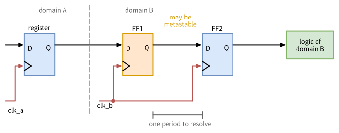
clk_b later, so FF1 has almost a whole period to resolve. Only the output of FF2 reaches the logic of domain B.
sync/rtl/sync_2ff.sv
// SPDX-FileCopyrightText: 2026 Simon Dorrer
// SPDX-License-Identifier: Apache-2.0
// Description: Two-flip-flop synchronizer. Brings WIDTH independent
// single-bit signals from another clock domain into the domain of
// clk_i. Each bit may arrive one cycle later than the others, so a
// bus must change only one bit at a time (Gray code).

`default_nettype none

module sync_2ff #(
  parameter int unsigned WIDTH = 1
) (
  input  logic             clk_i,
  input  logic             rst_ni,
  input  logic [WIDTH-1:0] d_i,   // from the other clock domain
  output logic [WIDTH-1:0] q_o
);

  logic [WIDTH-1:0] meta_q;  // may be metastable, never use it

  always_ff @(posedge clk_i or negedge rst_ni) begin
    if (!rst_ni) begin
      meta_q <= '0;
      q_o    <= '0;
    end else begin
      meta_q <= d_i;
      q_o    <= meta_q;
    end
  end

endmodule

`default_nettype wire
A synchronizer works only under a few rules:
- The signal leaves its domain from a register. Combinational logic in front of FF1 can glitch, and FF1 may capture the glitch.
- Nothing but FF2 reads FF1. Its output,
meta_q, may be metastable. Logic between the two flip-flops takes time away from \(t_r\). - Synchronize a signal once. Two synchronizers of the same signal may resolve differently, and their outputs then disagree for a cycle.
- Keep a level stable long enough. The destination must sample it at least once, so a level should last longer than a destination period plus the setup and hold window, in practice about 1.5 periods (Cummings 2008). From a fast to a slow domain, a one-cycle pulse can fall between two edges of the slow clock.
- Keep FF1 and FF2 close together in the layout, so that the wire between them takes as little time as possible. Some libraries offer synchronizer cells with a small \(\tau\), but SG13CMOS5L does not.
A pulse synchronizer solves the problem of the short pulse in the fourth rule. Each pulse in domain A toggles a level, the level crosses through a two-flip-flop synchronizer, and each change of the synchronized level becomes a one-cycle pulse in domain B:
sync/rtl/pulse_sync.sv
// SPDX-FileCopyrightText: 2026 Simon Dorrer
// SPDX-License-Identifier: Apache-2.0
// Description: Pulse synchronizer. A one-cycle pulse in domain A
// toggles a level, the level crosses through sync_2ff, and a change
// of the level gives a one-cycle pulse in domain B. Two pulses in A
// must be more than about 1.5 periods of clk_b_i apart.

`default_nettype none

module pulse_sync (
  input  logic clk_a_i,
  input  logic rst_a_ni,
  input  logic pulse_a_i,  // one-cycle pulses in domain A
  input  logic clk_b_i,
  input  logic rst_b_ni,
  output logic pulse_b_o   // one-cycle pulses in domain B
);

  logic tgl_a_q, tgl_b, tgl_b_q;

  // Domain A: every pulse toggles the level
  always_ff @(posedge clk_a_i or negedge rst_a_ni) begin
    if (!rst_a_ni) begin
      tgl_a_q <= 1'b0;
    end else if (pulse_a_i) begin
      tgl_a_q <= ~tgl_a_q;
    end
  end

  sync_2ff u_sync (
    .clk_i (clk_b_i),
    .rst_ni(rst_b_ni),
    .d_i   (tgl_a_q),
    .q_o   (tgl_b)
  );

  // Domain B: every change of the level is a pulse
  always_ff @(posedge clk_b_i or negedge rst_b_ni) begin
    if (!rst_b_ni) begin
      tgl_b_q <= 1'b0;
    end else begin
      tgl_b_q <= tgl_b;
    end
  end

  assign pulse_b_o = tgl_b ^ tgl_b_q;

endmodule

`default_nettype wire
Each toggled level must then obey the level rule above, so two pulses must be more than about 1.5 destination periods apart. The testbench sync/tb/tb_pulse_sync.sv sends 1000 one-cycle pulses from a 10 ns into a 14.3 ns domain, five cycles apart, i.e., 50 ns, well above 1.5 periods of the destination (about 21 ns). All 1000 arrive through pulse_sync. A plain synchronizer of the pulse itself, with an edge detector behind it, catches only 699, about 10/14.3 of them, the chance that an edge of clk_b falls inside the 10 ns pulse:
cd /foss/designs/vlsi-design/content/cdc/code/sync
iverilog -g2012 -o sim.vvp rtl/pulse_sync.sv rtl/sync_2ff.sv \
  tb/tb_pulse_sync.sv
vvp -n sim.vvp
TipExercise: How Long Until It Fails?
All commands start in the folder content/cdc/code/meta.
- Run the measurement in the slow corner,
python3 dff_meta.py slow, which takes a few minutes. Compare \(t_\text{cq0}\), \(\tau\), and \(T_0\) with the typical corner. Why does \(\tau\) change in this direction? - A signal from another clock domain changes 10 million times per second and is sampled at 250 MHz. Its first flip-flop drives 3 ns of logic in front of the next flip-flop. Compute the MTBF in the typical and in the slow corner. Take \(\tau\) and \(T_0\) from the measurement, and the clock-to-output delay and the setup time from the library, as STA does: 0.207 ns and 0.127 ns in the typical corner (Table 36). For the slow corner, run
CORNER=slow_1p08V_125C sta -no_init -exit ff.tclin/foss/designs/vlsi-design/content/sequential/code/ff, and take the larger of the two values of each (QandDrising and falling). - Compute the MTBF of a two-flip-flop synchronizer under the same conditions, in both corners.
- Is the two-flip-flop synchronizer good enough in the slow corner? By which factor does a third flip-flop raise the MTBF in the slow corner, and to how many years? At which clock frequency would two flip-flops reach an MTBF of 100 years in the slow corner?
Before continuing, please finish the previous exercise. Once you are done, compare with the solution below.
TipSolution: How Long Until It Fails?
- In the slow corner (slow transistors, 1.08 V, 125 °C), \(t_\text{cq0}\) = 330.7 ps, \(\tau\) = 158.7 ps, and \(T_0\) = 43.4 ps, against 220.4 ps, 85.9 ps, and 23.5 ps in the typical corner. Near the critical point, each decade adds about 365 ps instead of 198 ps. \(\tau\) is the capacitance of the latch loop divided by its transconductance. Slow transistors at a lower supply and a higher temperature deliver less current, so the loop amplifies more slowly.
- The library gives 0.305 ns and 0.208 ns in the slow corner. With 3 ns of logic, \(t_r = 4 - 0.207 - 3 - 0.127 = 0.666\) ns in the typical corner. The denominator is \(23.5\,\text{ps} \cdot 250\,\text{MHz} \cdot 10\,\text{MHz} = 58{,}750\) per second, and \(e^{666/85.9} = 2.3 \cdot 10^3\), so the MTBF is 0.040 s. In the slow corner, \(t_r = 4 - 0.305 - 3 - 0.208 = 0.487\) ns, the denominator is 108,500 per second, and the MTBF is 0.20 ms. The design fails 25 times per second, or about 5000 times per second in the slow corner.
- With a second flip-flop right behind the first, \(t_r\) = 3.666 ns in the typical corner, and the MTBF is \(5.83 \cdot 10^{13}\) s, i.e., \(1.85 \cdot 10^{6}\) years. In the slow corner, \(t_r\) = 3.487 ns gives \(3.21 \cdot 10^{4}\) s, only 8.9 hours.
- No, in the slow corner, each synchronizer fails on average every 9 hours. Even the bare schematic, whose \(\tau\) is too small, gives only 8.5 years. A third flip-flop gives the second one the same resolution time of 3.487 ns and multiplies the MTBF by \(e^{3487/158.7} = 3.5 \cdot 10^{9}\), to \(3.5 \cdot 10^{6}\) years. Two flip-flops reach 100 years only at a period of 5.767 ns, i.e., at 173 MHz instead of 250 MHz. Design synchronizers for the slow corner, where \(\tau\) is largest, and for the largest \(\tau\) the parasitics allow.
8.5 Crossing with Several Bits
A bus whose bits can change at the same time cannot cross through one synchronizer per bit. Each bit resolves on its own, so when several bits change at the same time, the destination can see a mix of old and new bits for a cycle, a value that the source never sent. A binary counter that steps from 7 to 8, i.e., from 0111 to 1000, changes all four bits and may arrive as any value from 0 to 15. There are three ways out:
- Gray code for counters and pointers. Consecutive values differ in exactly one bit, so the destination sees either the old or the new value, never a mix. The Gray code of a binary value \(b\) is \(g = b \oplus (b \gg 1)\), i.e.,
000,001,011,010,110,111,101,100for 0 to 7, and back to binary, bit \(i\) is the XOR of all bits of \(g\) from bit \(i\) upward. - A handshake for data words that change rarely. The source puts the word on the bus, keeps it stable, and toggles a request, which crosses through a synchronizer. When the destination sees the request, the word has been stable for several cycles, and the destination captures it and toggles an acknowledge back. The source changes the word only after the acknowledge has come back. Only the two control bits cross through synchronizers, at the price of several cycles per word.
- An asynchronous FIFO for data streams (Section 8.6).
An RTL simulation cannot show these problems by itself, because metastability is an analog effect that an RTL simulator does not model. The model sync/sim/sync_2ff_meta.sv replaces sync/rtl/sync_2ff.sv in a testbench. It has the same module name and ports, and it injects metastability: a bit of d_i that changed less than 1 ns before the clock edge resolves randomly to its old or its new value. The window is far wider than the real one, so that a crossing bug shows up within a few thousand cycles instead of years. At the end of a simulation, the model reports in how many samples at least one bit took its old value.
TipExercise: Count Across Clock Domains
All commands start in the folder content/cdc/code/gray. The module rtl/cnt_cross_bin.sv has a 4-bit counter in domain A that increments in every cycle, and reads it in domain B through one synchronizer per bit. The testbench tb/tb_cnt_cross.sv runs domain A at 10 ns and domain B at 13.7 ns for 5000 cycles of domain B, and it reports an error whenever the count in domain B advances by more than 2 in a cycle. The folder holds the reference solution rtl/cnt_cross_gray.sv, so move it out of the way first: cd /foss/designs/vlsi-design/content/cdc/code/gray, then mv rtl/cnt_cross_gray.sv cnt_cross_gray_solution.sv.
Simulate
cnt_cross_binwith../sync/rtl/sync_2ff.svand with the model:iverilog -g2012 -DDUT=cnt_cross_bin -o sim.vvp \ rtl/cnt_cross_bin.sv ../sync/rtl/sync_2ff.sv tb/tb_cnt_cross.sv vvp -n sim.vvp iverilog -g2012 -DDUT=cnt_cross_bin -o sim.vvp \ rtl/cnt_cross_bin.sv ../sync/sim/sync_2ff_meta.sv \ tb/tb_cnt_cross.sv vvp -n sim.vvpHow many errors does each run report, and in how many samples does the model report a bit at its old value? For the first two wrong counts of the second run, find the counter step that FF1 sampled, and which bits took their old and which their new value. Hint: the count advances by 1 or 2 per cycle of domain B.
Draw a block diagram of a counter that crosses in Gray code: the counter and the conversion to Gray code in domain A, the synchronizers, and the conversion back in domain B. Which signals are registers?
Write
rtl/cnt_cross_gray.svwith the ports ofcnt_cross_bin, check it withverilator --lint-only -Wall rtl/cnt_cross_gray.sv ../sync/rtl/sync_2ff.sv, and simulate it with the model, i.e., the secondiverilogcommand of step 1 with-DDUT=cnt_cross_grayandrtl/cnt_cross_gray.sv. How many errors remain?
Before continuing, please finish the previous exercise. Once you are done, compare with the solution below.
TipSolution: Count Across Clock Domains
- With
rtl/sync_2ff.sv, the testbench reports5000 cycles of domain B, 0 errors. In an RTL simulation, every bit that changes at an edge ofclk_ais sampled consistently by the next edge ofclk_b, so the binary crossing looks correct. With the model, it reports 224 errors, and in 334 of 5001 samples, at least one bit took its old value. The first wrong counts are 7 after 4 at 90.0 ns, 12 after 14 at 350.4 ns, and 1 after 12 at 364.1 ns. One cycle of domain B earlier, at 335.65 ns, FF1 sampled the counter 0.65 ns after it had stepped from 15 (1111) to 0 (0000), and all four bits changed. The two upper bits resolved to their old, the two lower ones to their new value,1100, i.e., 12, a value the counter had four counts earlier. The count 1 at 364.1 ns is correct again, but it is flagged because it follows the wrong 12. At 90.0 ns, the step from 5 (0101) to 6 (0110) arrived as0111, i.e., 7: bit 0 kept its old 1, and bit 1 took its new 1. - In domain A, the counter
cnt_a_qand a registergray_a_qthat holds its Gray code. The register is the source of the synchronizers, so the XOR gates in front of it cannot reach domain B with a glitch. In domain B, the four synchronizers and the combinational conversion back to binary behind them. The Gray register delays the count by one cycle of domain A, which does not matter for a counter that crosses domains. - The reference solution:
gray/rtl/cnt_cross_gray.sv
// SPDX-FileCopyrightText: 2026 Simon Dorrer
// SPDX-License-Identifier: Apache-2.0
// Description: The counter of cnt_cross_bin, crossing in Gray code.
// Only one bit changes per count, so domain B sees either the old or
// the new value, never a mix.

`default_nettype none

module cnt_cross_gray #(
  parameter int unsigned W = 4
) (
  input  logic         clk_a_i,
  input  logic         rst_a_ni,
  input  logic         clk_b_i,
  input  logic         rst_b_ni,
  output logic [W-1:0] cnt_b_o
);

  logic [W-1:0] cnt_a_q, gray_a_q, gray_b;

  // Domain A: the counter and its Gray code in a register, so that
  // no logic glitch reaches the synchronizer
  always_ff @(posedge clk_a_i or negedge rst_a_ni) begin
    if (!rst_a_ni) begin
      cnt_a_q  <= '0;
      gray_a_q <= '0;
    end else begin
      cnt_a_q  <= cnt_a_q + 1'b1;
      gray_a_q <= cnt_a_q ^ (cnt_a_q >> 1);
    end
  end

  // Into domain B, then back to binary
  sync_2ff #(.WIDTH(W)) u_sync (
    .clk_i (clk_b_i),
    .rst_ni(rst_b_ni),
    .d_i   (gray_a_q),
    .q_o   (gray_b)
  );

  always_comb begin
    for (int i = 0; i < W; i++) begin
      cnt_b_o[i] = ^(gray_b >> i);
    end
  end

endmodule

`default_nettype wire
With the model, no error remains in 5000 cycles, although a bit took its old value in 260 samples. Each of them is one bit of a Gray step, so the count is the old or the new value, which the testbench accepts.
8.6 The Asynchronous FIFO
The FIFO of Section 4 has one clock. Its asynchronous version connects two clock domains: the producer pushes in the write domain, the consumer pops in the read domain (Figure 42). The memory is written with the write clock and read with the read clock. Each pointer exists in binary, to address the memory, and in Gray code, in a register, to cross into the other domain (Cummings 2002).
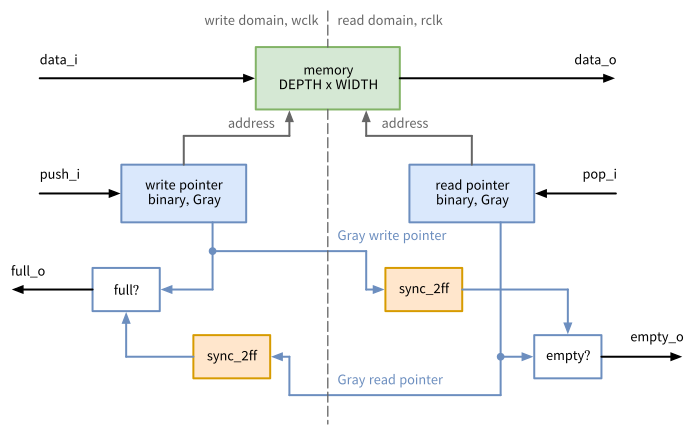
fifo/rtl/async_fifo.sv
// SPDX-FileCopyrightText: 2026 Simon Dorrer
// SPDX-License-Identifier: Apache-2.0
// Description: Asynchronous FIFO between a write and a read clock
// domain, with first-word fall-through like the FIFO of chapter 4.
// The pointers cross the domains in Gray code through sync_2ff.

`default_nettype none

module async_fifo #(
  parameter int unsigned WIDTH = 8,
  parameter int unsigned DEPTH = 4  // power of two, at least 4
) (
  // Write domain
  input  logic             wclk_i,
  input  logic             wrst_ni,
  input  logic             push_i,
  input  logic [WIDTH-1:0] data_i,
  output logic             full_o,
  // Read domain
  input  logic             rclk_i,
  input  logic             rrst_ni,
  input  logic             pop_i,
  output logic [WIDTH-1:0] data_o,
  output logic             empty_o
);

  localparam int unsigned AW = $clog2(DEPTH);

  logic [AW:0]      wbin_q, wgray_q, wbin_d;  // write pointer
  logic [AW:0]      rbin_q, rgray_q, rbin_d;  // read pointer
  logic [AW:0]      rgray_w, wgray_r;  // synchronized into the other
  logic [WIDTH-1:0] mem_q [DEPTH];
  logic             push, pop;

  // Write domain: the pointer in binary and in Gray code
  always_ff @(posedge wclk_i or negedge wrst_ni) begin
    if (!wrst_ni) begin
      wbin_q  <= '0;
      wgray_q <= '0;
    end else begin
      wbin_q  <= wbin_d;
      wgray_q <= wbin_d ^ (wbin_d >> 1);
    end
  end

  always_ff @(posedge wclk_i) begin
    if (push) begin
      mem_q[wbin_q[AW-1:0]] <= data_i;
    end
  end

  // Read domain
  always_ff @(posedge rclk_i or negedge rrst_ni) begin
    if (!rrst_ni) begin
      rbin_q  <= '0;
      rgray_q <= '0;
    end else begin
      rbin_q  <= rbin_d;
      rgray_q <= rbin_d ^ (rbin_d >> 1);
    end
  end

  // Each Gray pointer into the other domain
  sync_2ff #(.WIDTH(AW + 1)) u_sync_r2w (
    .clk_i (wclk_i),
    .rst_ni(wrst_ni),
    .d_i   (rgray_q),
    .q_o   (rgray_w)
  );

  sync_2ff #(.WIDTH(AW + 1)) u_sync_w2r (
    .clk_i (rclk_i),
    .rst_ni(rrst_ni),
    .d_i   (wgray_q),
    .q_o   (wgray_r)
  );

  // Full: the write pointer is one lap ahead of the read pointer,
  // which in Gray code inverts the two upper bits
  assign full_o  = (wgray_q == {~rgray_w[AW:AW-1], rgray_w[AW-2:0]});
  assign empty_o = (rgray_q == wgray_r);
  assign data_o  = mem_q[rbin_q[AW-1:0]];

  always_comb begin
    push   = push_i && !full_o;
    pop    = pop_i && !empty_o;
    wbin_d = push ? wbin_q + 1'b1 : wbin_q;
    rbin_d = pop ? rbin_q + 1'b1 : rbin_q;
  end

endmodule

`default_nettype wire
As in Section 4, the pointers have one bit more than the address. The FIFO is empty when the read pointer equals the write pointer, and full when the write pointer is one lap of DEPTH entries ahead of the read pointer. In binary, one lap ahead means the same address with the wrap bit inverted. In Gray code, the codes of \(n\) and \(n + \text{DEPTH}\) differ in their two upper bits, e.g., 000 and 110 for 0 and 4, hence the inversion in full_o.
Each domain computes its flag from its own pointer and the synchronized pointer of the other domain, which lags one to three cycles of its own clock behind. So full_o may still be high although the read domain has already freed an entry, and empty_o although the write domain has already filled one: the flags are pessimistic, but they are never low when the FIFO is full or empty. With Gray code, the synchronized pointer is always either the old or the new value of the pointer. A binary pointer could arrive as a mix of both for a cycle and make the fill level jump. This FIFO even survives that in simulation, because each side moves at most one entry per cycle and the wrong value lasts only one cycle, but an output with the fill level, an almost-full flag, or a read of several entries at once would fail. Gray pointers rule it out. The memory needs no synchronizer: the read domain reads an entry only after the synchronized write pointer shows that it was written, more than one read clock period after the write, so the entry is stable when it is read. In a chip, wrst_ni and rrst_ni each come from a reset synchronizer of their own domain (Section 8.8), and both domains must be reset together.
The testbench fifo/tb/tb_async_fifo.sv runs the write domain at 10 ns and the read domain at 14.3 ns, pushes and pops at random, and checks every popped word against a scoreboard. With the metastability model in place of the synchronizer, it reports 9397 pushed, 9395 popped, 0 errors, while at least one bit took its old value in 481 of 20,000 samples of the read pointer and in 367 of 13,986 samples of the write pointer:
cd /foss/designs/vlsi-design/content/cdc/code/fifo
iverilog -g2012 -o sim.vvp rtl/async_fifo.sv \
  ../sync/sim/sync_2ff_meta.sv tb/tb_async_fifo.sv
vvp -n sim.vvp
8.7 Constraints for Clock Domain Crossings
The constraints of async_fifo define one clock per domain, and the ports of each domain refer to their own clock:
fifo/syn/async_fifo.sdc
# SPDX-FileCopyrightText: 2026 Simon Dorrer
# SPDX-License-Identifier: Apache-2.0
# Description: Timing constraints of async_fifo: a write clock of
# 100 MHz and an unrelated read clock of about 70 MHz, each with the
# ports of its own domain.

create_clock -name wclk -period 10.0 [get_ports wclk_i]
create_clock -name rclk -period 14.3 [get_ports rclk_i]
set_clock_transition 0.1 [all_clocks]
set_clock_uncertainty 0.1 [all_clocks]

# The ports of each domain refer to their own clock
set w_in [get_ports {wrst_ni push_i data_i*}]
set r_in [get_ports {rrst_ni pop_i}]
set_input_delay 1.0 -clock wclk $w_in
set_input_delay 1.0 -clock rclk $r_in
set_output_delay 1.0 -clock wclk [get_ports full_o]
set_output_delay 1.0 -clock rclk [get_ports {data_o* empty_o}]
set_driving_cell -lib_cell sg13cmos5l_buf_2 -pin X $w_in
set_driving_cell -lib_cell sg13cmos5l_buf_2 -pin X $r_in
set_load 0.01 [all_outputs]
Without further constraints, STA treats two clocks as synchronous. It searches the edges of both clocks over their common period, here 1430 ns, for the tightest pair. Synthesized as in the earlier chapters (134 cells, 3979 µm²), async_fifo gives this report:
cd /foss/designs/vlsi-design/content/cdc/code/fifo
yosys -p "read_verilog -sv ../sync/rtl/sync_2ff.sv \
  rtl/async_fifo.sv; synth -top async_fifo; flatten; \
  dfflibmap -liberty $LIB; abc -constr $CONSTR -liberty $LIB; \
  opt_clean; stat -liberty $LIB; \
  write_verilog -noattr async_fifo.nl.v"
sta -no_init -exit syn/sta.tcl
The worst path of the group rclk runs from a memory flip-flop, launched by wclk at 100.0 ns, to data_o[0], captured by rclk at 100.1 ns, and fails with a slack of -1.414 ns. The worst path of the group wclk ends at a synchronizer flip-flop of the read pointer and fails with -0.382 ns. Both are meaningless: the clocks have no fixed phase, the edges come arbitrarily close to each other anyway, and the synchronizers and the protocol of the FIFO take care of it.
set_clock_groups -asynchronous tells STA that the clocks are unrelated, and it then times no path between them:
set_clock_groups -asynchronous -group wclk -group rclkWith CDC=1 sta -no_init -exit syn/sta.tcl, the script adds this line, the crossing paths disappear (No paths found), and the worst slacks are 12.488 ns in rclk and 8.171 ns in wclk. The constraint hides every crossing, including one without a synchronizer, so STA cannot check crossings at all. Commercial CDC tools check the structure of every crossing. In the open-source flow, design rules do the job: every crossing goes through one of a few synchronizer modules, such as sync_2ff. A search for their instances finds the synchronizers, but not a crossing without one. For that, list the endpoints of all crossing paths before the clock groups hide them:
report_checks -from [get_clocks wclk] -to [get_clocks rclk] \
  -group_path_count 100 -endpoint_path_count 1 -format end
Together with the other direction, async_fifo has 14 such endpoints: the 8 outputs data_o, which the protocol of the FIFO protects, and the 6 first flip-flops of the two synchronizers. Any other endpoint would be a crossing without a synchronizer.
NoteOpenCDC
The IIC-OSIC-TOOLS image also contains OpenCDC (opencdc), an open-source tool that checks the structure of clock domain crossings in RTL. It is still at an early stage and does not yet judge all designs of this chapter correctly, so this course stays with the design rules and the endpoint list above.
A stricter alternative limits the delay of every crossing path instead of removing it, so that the bits of a Gray pointer arrive within one period of their source clock of each other, and the memory data within less than a read period, before the read domain can use the entry:
set_max_delay 10.0 -ignore_clock_latency \
  -from [get_clocks wclk] -to [get_clocks rclk]
set_max_delay 10.0 -ignore_clock_latency \
  -from [get_clocks rclk] -to [get_clocks wclk]
set_false_path -hold -from [get_clocks wclk] -to [get_clocks rclk]
set_false_path -hold -from [get_clocks rclk] -to [get_clocks wclk]
The limit of 10 ns is the period of the write clock, the source of the write pointer, which is the tighter case. -ignore_clock_latency leaves the clock latencies out of the limit, which after clock tree synthesis differ between the two unrelated clock trees, and it changes nothing for ideal clocks. With CDC=2 sta -no_init -exit syn/sta.tcl, the script uses these lines instead of the clock groups. OpenSTA reports the crossing paths in the path group path delay, the path to data_o[0] with a slack of 8.586 ns against the limit of 10 ns. Without the two false paths, it would still check hold between the clocks, which means as little as the setup checks before.
8.8 Resets
The asynchronous reset of our designs (Section 2.5.6) acts at once, without a clock. Asserting it at any moment is safe: every flip-flop goes into reset. Releasing it is a crossing. The reset comes from a pin or from a power-on-reset circuit, which holds the reset low until the supply has settled, asynchronous to the clock, and when its release falls into the window of the recovery and removal checks (Section 6.3), some flip-flops leave the reset at one clock edge and others one edge later. The design then starts in a state that the RTL never reaches.
A reset synchronizer asserts the reset of a clock domain at once, asynchronously, and releases it synchronously, at a clock edge. Its output drives the reset inputs of all registers of the domain, so that they all leave the reset at the same clock edge. Every clock domain needs its own reset synchronizer. The reset input itself must be free of glitches, because even a short pulse resets the design asynchronously. A chip therefore takes it from a power-on-reset circuit or from a filtered pin, whose input stage ignores pulses shorter than a set time.
TipExercise: Release the Reset
All commands start in the folder content/cdc/code/reset. It holds the reference solution rtl/rst_sync.sv, so move it out of the way first: cd /foss/designs/vlsi-design/content/cdc/code/reset, then mv rtl/rst_sync.sv rst_sync_solution.sv.
Draw the reset synchronizer with the ports
clk_i,rst_ni, andrst_no, and a timing diagram ofclk_i,rst_ni, the internal flip-flop, andrst_nofor a reset that falls between two clock edges and rises shortly before a rising edge. Hint: start fromsync_2ff. What must the first flip-flop load after the release?Write
rtl/rst_sync.sv, check it withverilator --lint-only -Wall rtl/rst_sync.sv, and simulate it with the testbench:iverilog -g2012 -o sim.vvp rtl/rst_sync.sv tb/tb_rst_sync.sv vvp -n sim.vvpWhen does
rst_norise after the release, and how many errors does the testbench report?The module
rtl/bs_reg_rs.svputs your synchronizer in front of the barrel shifter between two registers of Section 6.7. Synthesize it and run the timing script with the constraints ofbs_reg(Section 6.6):yosys -p "read_verilog -sv \ ../../../verification/code/barrel_shift/rtl/barrel_shift.sv \ ../../../sequential/code/bs_reg/rtl/bs_reg.sv \ rtl/rst_sync.sv rtl/bs_reg_rs.sv; synth -top bs_reg_rs; \ flatten; dfflibmap -liberty $LIB; \ abc -constr $CONSTR -liberty $LIB; opt_clean; \ stat -liberty $LIB; write_verilog -noattr bs_reg_rs.nl.v" sta -no_init -exit syn/sta.tclWhat is the slack of the worst recovery path now? How long does its startpoint need to drive its load, compared with the clock-to-output delay in Table 36, and what does that do to the recovery time? Compare the minimum periods with those of
bs_regin Section 6.7. What doesreport_check_typesreport, and why did synthesis not fix it?Which checks does STA still make on the input
rst_ni, and do they mean anything? The script reports them at its end. Copysyn/bs_reg_rs.sdctosyn/bs_reg_rs_rst.sdc, add the constraint that fits, and runSDC=syn/bs_reg_rs_rst.sdc sta -no_init -exit syn/sta.tcl. Which checks remain in the groupasynchronous, and does the minimum period change?
Before continuing, please finish the previous exercise. Once you are done, compare with the solution below.
TipSolution: Release the Reset
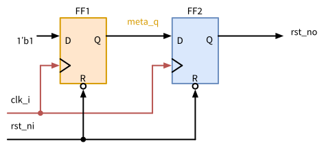
rst_ni resets both at once. After its release, the first flip-flop loads the constant 1 at the next rising edge of clk_i, possibly metastable, and the second one passes it on one period later, as rst_no for all registers of the clock domain.
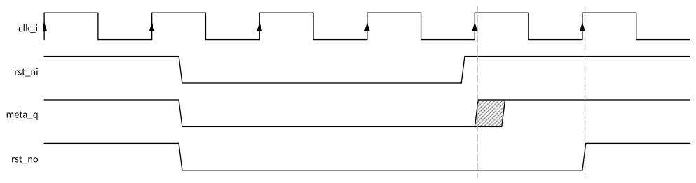
rst_ni falls between two clock edges, and meta_q and rst_no fall at once. rst_ni rises within the recovery time before a rising edge (dashed), so meta_q may become metastable (crossed). Here it settles to 1, and rst_no rises one period later. If it settled to 0, rst_no would rise one period later still, again at a clock edge for all registers of the domain.
- The reference solution:
reset/rtl/rst_sync.sv
// SPDX-FileCopyrightText: 2026 Simon Dorrer
// SPDX-License-Identifier: Apache-2.0
// Description: Reset synchronizer. Asserts the reset of a clock
// domain at once, asynchronously, and releases it synchronously, two
// or, if the first flip-flop resolves late, three rising edges of
// clk_i after rst_ni rises.

`default_nettype none

module rst_sync (
  input  logic clk_i,
  input  logic rst_ni,  // asynchronous reset, e.g., from a pad
  output logic rst_no   // reset of the clock domain of clk_i
);

  logic meta_q;  // may be metastable after the release

  always_ff @(posedge clk_i or negedge rst_ni) begin
    if (!rst_ni) begin
      meta_q <= 1'b0;
      rst_no <= 1'b0;
    end else begin
      meta_q <= 1'b1;
      rst_no <= meta_q;
    end
  end

endmodule

`default_nettype wire
The testbench prints that rst_no is low 0.1 ns after rst_ni falls at 42 ns, between two clock edges, and that after the release at 64.8 ns, 0.2 ns before the edge at 65 ns, rst_no rises at 75 ns, the second rising edge after the release, with 0 errors.
bs_reg_rshas 927 cells, 15,343 µm², and 73 flip-flops, two more thanbs_reg. The worst recovery path now starts at the second flip-flop of the synchronizer, whose output drives theRESET_Bpins of all 71 registers. The flip-flop needs 1.375 ns for that, against its normal 0.207 ns. The slew of 1.721 ns raises the recovery time to 0.451 ns, and the slack is 2.074 ns. The release of the reset is now a path between two registers of the same clock, andreport_clock_min_periodincludes it: \(1.375 + 0.451 + 0.1 = 1.93\) ns (519 MHz), with and without the port paths. Inbs_reg, the paths between the registers needed 1.69 ns, and the reset input with its input delay limited the block to 2.02 ns.report_check_typesreports the output of the synchronizer flip-flop with 0.43 pF against a limit of 0.30 pF. The load lies beyond the last index of the tables, so the delay and the slew above are extrapolated (Section 5.5). ABC buffers only the logic it maps, and this net runs from a flip-flop straight to flip-flops. The layout flow buffers it like any net with a large fanout (Section 10).- STA still checks the recovery and the removal of the two synchronizer flip-flops against
rst_niwith its input delay of 1 ns, with slacks of 2.768 and 1.007 ns. These checks mean nothing: the release ofrst_niis asynchronous, and violating the recovery time of the first flip-flop is exactly the case that the synchronizer handles. The second flip-flop loads the 0 of the first one at the first edge after the release, so its output is the same whether it leaves the reset at this edge or the next. The constraint is a false path:
set_false_path -from [get_ports rst_ni]With it, STA finds no path from rst_ni anymore, the remaining checks of the group asynchronous all start at the synchronizer, with a worst removal slack of 1.341 ns, and the minimum period stays at 1.93 ns.
8.9 Summary
- Registers driven by one clock form a clock domain. Paths between asynchronous clocks, and from asynchronous input pins such as a button or a chip on its own clock, cross domains, and STA cannot check them.
- A flip-flop whose data changes inside its window becomes metastable and resolves with the time constant \(\tau\). In ngspice, with an estimate of its wiring capacitance,
dfrbpq_1has \(\tau\) = 85.9 ps and \(T_0\) = 23.5 ps in the typical corner. The MTBF \(e^{t_r/\tau}/(T_0 f_\text{clk} f_\text{data})\) depends exponentially on the resolution time, so design for the slow corner. - A two-flip-flop synchronizer gives the first flip-flop a period to resolve. It needs a register in the source domain, no logic between the flip-flops, and one synchronizer per signal. A third flip-flop multiplies the MTBF by about \(e^{(T - t_\text{cq0} - t_\text{su})/\tau}\). A pulse crosses as a toggled level.
- A bus whose bits can change at the same time cannot cross through one synchronizer per bit. Counters and pointers cross in Gray code, rare data words with a handshake, data streams through an asynchronous FIFO with Gray pointers, whose flags may be pessimistic but are never low when the FIFO is full or empty.
- RTL simulation does not show metastability. A synchronizer model with metastability injection makes crossing bugs visible.
- STA needs
set_clock_groups -asynchronousorset_max_delay -ignore_clock_latencyfor the paths between asynchronous clocks, and the structure of the crossings must be checked by review or a CDC tool. - A reset synchronizer asserts the reset asynchronously and releases it synchronously, one per clock domain, and the input reset is a false path.
In Section 9, the design gets scan chains, and the clock domains and synchronizers of this chapter need special care in test mode.
9 Design for Test (DFT)
A chip that passed every simulation, every timing check, and the equivalence check can still fail on the bench: a particle on the wafer shorted two wires, a via did not open, a transistor does not switch. Verification checks that the design is right (Section 4). The test checks that a manufactured die equals the design. It runs on every die, it may take a few seconds at most, and it must find almost every defect. For a design with thousands of flip-flops, this is only possible if the design was prepared for it, which is called design for test (DFT). This chapter introduces the fault models that turn defects into something a tool can count, the generation of tests, scan chains, which make every flip-flop accessible to the tester, and the design rules that keep a design testable.
Note
All code of this chapter is available in the folder content/dft/code of the course repository: transistor faults of a NOR gate in ngspice in transistor/, a small gate-level netlist, its fault classes, and the test generation with a SAT solver in atpg/, the scan insertion with and without placement, the conversion of test vectors into scan patterns, the scan testbench, and the equivalence check after scan insertion in scan/, and the barrel shifter with a reset synchronizer and a test mode in reset/. All numbers in this chapter come from the IIC-OSIC-TOOLS image 2026.10 (ngspice 47, Yosys 0.70, OpenROAD 26Q4 as the standalone openroad, OpenSTA 3.1.0, Fault 0.9.4, Icarus Verilog 14.0) and SG13CMOS5L, in the typical corner. The script scripts/check_dft.sh reproduces all of them: run bash scripts/check_dft.sh in the container from the root of the repository.
For the exercises, clone the course repository into your designs folder once, if you have not done so yet:
cd /foss/designs
git clone https://github.com/iic-jku/vlsi-design.git
In every new terminal, define the paths of the typical-corner library, of the ABC constraint file of Section 5.7, and of the Verilog models of the cells, and set two variables for the tool Fault of Section 9.4:
LIB=$PDK_ROOT/ihp-sg13cmos5l/libs.ref/sg13cmos5l_stdcell/lib
LIB=$LIB/sg13cmos5l_stdcell_typ_1p20V_25C.lib
CONSTR=/foss/designs/vlsi-design/content/synthesis_lib/code
CONSTR=$CONSTR/synth/abc.constr
CELLS=$PDK_ROOT/ihp-sg13cmos5l/libs.ref/sg13cmos5l_stdcell/verilog
export SWIFT_DETERMINISTIC_HASHING=1 FAULT_THREADS=4
Fault is written in Swift, whose hash tables take a new random seed in every run, so its compaction keeps a different set of vectors from run to run. The first variable fixes the seed, so that your results match those of the book. The second limits Fault to four threads. Fault 0.9.4 still stops now and then with Illegal instruction, a race between its threads that hits more often the busier the machine is: on an idle machine, none of 20 runs with four threads crashed, on a machine loaded three times over, 18 of 20 did. Run the command again, the vectors do not change.
9.1 Learning Objectives
After this chapter, you will be able to:
- explain why every manufactured die is tested, relate yield, fault coverage, and defect level, and tell catastrophic from parametric yield loss
- model defects as stuck-at, transition, bridging, and transistor faults, collapse equivalent faults, and explain IDDQ testing
- find a test for a fault by hand with the D-algorithm and with a SAT solver, and recognize untestable faults
- explain how scan makes a sequential circuit testable, insert scan chains with OpenROAD with and without a placement, and compute the test time
- generate test vectors with Fault and apply them through a scan chain in simulation
- apply the design rules for testability to clocks, clock gates, resets, clock domains, and the scan chain itself
- name the tests beyond scan: at-speed test, built-in self-test, and boundary scan
9.2 Why Test?
Manufacturing is never perfect, and the share of good dies on a wafer, the yield \(Y\), never reaches 100 %. Particles on the wafer and defects in the lithography cause shorts between wires, open vias, and transistors that do not switch. Such random defects make a die fail outright, which is the catastrophic yield loss. Variations of the process instead make a die without any defect too slow or too leaky, which is the parametric yield loss. The design limits it with the corners of Section 5.6 and the timing margins of Section 6.5. The yield falls with the die area and rises as a process matures, but every die must be tested before it is shipped. Verification asks whether the design is right, the test asks whether a die equals the design (Section 4.2). The test assumes that the design is correct, and it compares the responses of the die with those of the netlist.
Most chips are tested twice. The wafer test contacts the pads of each die with the needles of a probe card before the wafer is sawn, and the failing dies are recorded in a wafer map and never packaged. The final test repeats the test after packaging, because sawing, bonding, and molding add defects of their own. Over the lifetime of a population of chips, the failure rate has the shape of a bathtub (Figure 45): parts with weak spots fail early, then failures are rare and random for years, until wear-out sets in. Parts for cars or medical devices therefore often also run a burn-in at raised temperature and supply voltage, which makes weak parts fail before they are shipped. The tester, called automatic test equipment (ATE), applies the test. A computer runs the test program, which sets the timing of the vectors, and the pin electronics drive each pin and sample its response through a probe card or a socket. In every clock cycle, the tester drives a vector onto the inputs and compares the outputs with the expected values. Tester time is expensive, so the test of a die takes seconds at most, and every vector counts.
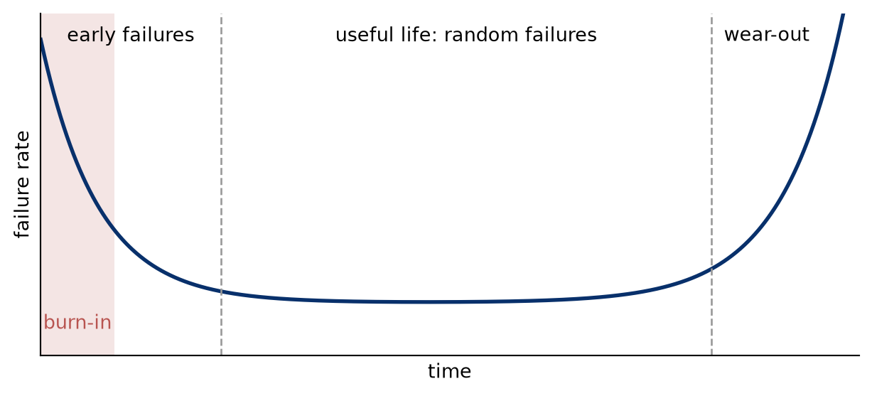
A defect that escapes the test costs more the later it is found. A rule of thumb says that the cost grows by about a factor of ten from step to step: on the wafer, in the package, on the board, and in the system of the customer, where a defective part in a car can mean a recall. The fault coverage \(T\) of a test is the share of the modeled faults that it detects (Section 9.3). With less than 100 %, some defective dies pass. The opposite error exists as well: a test whose limits are too tight, e.g., on the supply current or the speed, rejects good dies, which is called overkill. It costs yield, but no customer sees it. The defect level \(DL\), the share of defective dies among those that pass the test, follows from the yield and the coverage in the model of Williams and Brown (Williams and Brown 1981):
\[ DL = 1 - Y^{1-T} \]
With 80 % yield and 99 % coverage, 0.22 % of the shipped dies are defective, 2229 parts per million (ppm), or one in 449 (Figure 46). Customers in the automotive industry ask for defect levels of a few ppm. Even for 100 ppm at 80 % yield, the coverage must reach \(T = 1 - \ln(1 - DL)/\ln Y\) = 99.955 %, and at a lower yield, more still.
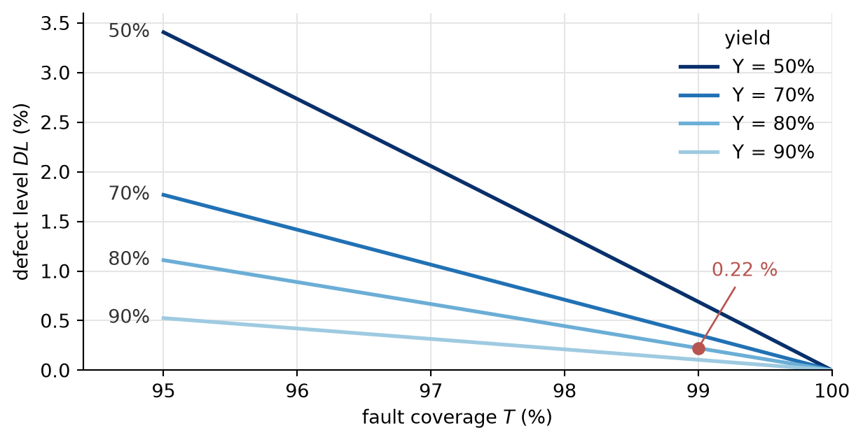
9.3 Fault Models
A test cannot target physical defects directly: their number is endless, and their effect depends on the layout. Instead, it targets faults, models of defects on the netlist that a tool can list and simulate (Bushnell and Agrawal 2000). The terms form a chain. A defect is the physical flaw, e.g., a short between two wires. A fault models it on the netlist, e.g., as a net stuck at 0. For some inputs, the fault causes an error, a wrong value at an output, and an error that reaches the application becomes a failure of the system. The test looks for errors at the outputs of the die, long before any failure.
The stuck-at fault model assumes that a net or a pin of a cell is fixed at 0 (stuck-at-0, s-a-0) or at 1 (stuck-at-1, s-a-1), while all cells keep their functions. The single stuck-at model assumes one fault at a time, so \(n\) fault sites give \(2n\) faults, whereas multiple faults would give \(3^n - 1\) combinations. The model is simple, yet a test that detects all single stuck-at faults also detects many other defects, because a short or an open usually forces some net to a wrong value for some input. The tool Fault of Section 9.4 counts every pin of every cell and every port bit, except the clock and the reset input, as a fault site.
Many faults are equivalent, i.e., exactly the same tests detect them. A stuck-at-1 at an input of an OR gate forces its output to 1, just like a stuck-at-1 at the output. Tools merge equivalent faults, which shortens the list (fault collapsing). A net that drives several cell inputs has fault sites on its stem, the net as a whole, and on each branch to one of the inputs, because a defect can cut off a single branch. For a netlist of AND, OR, NAND, NOR, and NOT gates, merging the faults that are equivalent within each gate leaves
\[ N = 2\,(P_O + F_O) + G_I - N_I \]
faults, with \(P_O\) primary outputs, the outputs of the design itself, \(F_O\) fanout stems, \(G_I\) inputs of all gates, inverters included, and \(N_I\) inverters (Wang et al. 2006). In large netlists, this removes about half of the faults. Some faults cannot be detected at all, because no input makes the faulty circuit behave differently from the good one, e.g., in redundant logic. Such a fault is untestable, like an equivalent mutant in Section 4.9. The fault coverage counts all faults, the test coverage leaves out the untestable ones, so it reaches 100 % when every detectable fault is detected.
Other fault models and test methods capture defects that the stuck-at model misses:
- Transition faults model a gate that is too slow: its output rises (slow-to-rise) or falls (slow-to-fall) too late. Their test needs two vectors: the first sets the old value, the second launches the transition, and the response is captured one clock period later, at the speed of the chip (Section 9.7). The test detects an extra delay only if it exceeds the slack that the path along which the two vectors propagate the transition has on this die at the test clock period (Section 6.5). Through a short path, only a large delay shows up, so timing-aware test generation tries to propagate the transition along the longest testable path through each fault site, to catch small delay defects as well. A transition fault models a local spot defect. Path delay faults (Smith 1985) model the sum of small extra delays along a whole path, e.g., from variations of the process. Each path has two such faults, one for a rising and one for a falling transition, and the number of paths can grow exponentially with the depth of the logic, so a test targets only the critical paths from the STA.
- Bridging faults short two nets. The result depends on the drivers: the stronger one wins, or the bridge acts like an AND or an OR of both nets. A test drives the two nets to opposite values. With \(n\) nets, \(n(n-1)/2\) pairs could short, so tools take only pairs of neighboring wires from the layout. Stuck-at tests detect many bridges as well. A test for net \(A\) stuck-at-0 drives \(A\) to 1. If it also drives the bridged net \(B\), which does not depend on \(A\), to 0, and \(B\) has the stronger driver, the bridge acts like the stuck-at fault, and the test detects it.
- Stuck-open and stuck-on faults model a transistor that never or always conducts. With a stuck-open transistor, the output of the CMOS gate floats for some inputs and keeps its last value, so the gate turns into a memory, and the test needs two vectors. For some inputs, a stuck-on transistor fights the transistors that should drive the output, which gives a level between the rails and a current from the supply to ground.
- IDDQ testing measures the quiescent supply current. A CMOS circuit at rest draws only its leakage current. A defect that connects the supply to ground in some states only, e.g., a bridge between two nets driven to opposite values, raises the current far above that in these states, which a current measurement after a few vectors finds, even when no output shows a wrong value. In large chips of modern processes, the leakage itself is high and varies from die to die, which hides the extra current.
TipExercise: Transistor Faults
All commands start in the folder content/dft/code/transistor. The script nor2_faults.py simulates the NOR gate sg13cmos5l_nor2_1 of the PDK in ngspice, with an inv_1 at its output Y. It applies the input vectors (A, B) = 00, 10, 11, 10, 00, 01, each for 2 ns, and prints Y and the output Z of the inverter at the end of each vector, and the quiescent supply current IDDQ of each vector from an operating point, i.e., after a long wait.
- Draw the transistor schematic of
nor2_1from its subcircuit in the filesg13cmos5l_stdcell.spiceinlibs.ref/sg13cmos5l_stdcell/spice/of the PDK, with the instance names of the transistors. - The NMOS transistor
XN0at inputAis stuck-open. For which input vector doesYfloat? Find a test of two vectors, and a sequence in which the same second vector does not detect the fault. - Check your answer with
python3 nor2_faults.py n_open, and compare withpython3 nor2_faults.py good. Why isYslightly above VDD in the vector where it floats? How long does the floating gate keep its value? WithHOLD=1and two vectors inSEQ, e.g.,HOLD=1 SEQ="00 01" python3 nor2_faults.py n_open, the script applies the first vector and then holds the second one for a second. Try your test and your sequence of step 2. - Instead,
XN0is stuck-on, or the PMOS transistorXP0at inputAis stuck-on: runpython3 nor2_faults.py n_onandpython3 nor2_faults.py p_on. For which vectors do transistors fight? Which of the two faults does a test of the logic values detect, and which one only IDDQ? Which level doesYtake in a fight, and why?
Before continuing, please finish the previous exercise. Once you are done, compare with the solution below.
TipSolution: Transistor Faults
- The two PMOS transistors connect
Yin series to VDD, the two NMOS transistors in parallel to VSS (Figure 47).
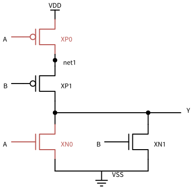
sg13cmos5l_nor2_1, as in the SPICE netlist of the PDK. The PMOS transistors XP0 and XP1 connect Y in series to VDD, and the NMOS transistors XN0 and XN1 in parallel to VSS. The faults of the exercise sit in the two transistors at input A, XP0 and XN0 (red).
With (
A,B) = 10,XP0is off,XN1is off, andXN0should pullYto 0, but it never conducts, soYfloats. The test 00 followed by 10 detects the fault: 00 setsYto 1, which the faulty gate keeps at 10, where the good gate gives 0. After 11 or 01,Yis already 0, and the faulty gate keeps the right value at 10 for the few nanoseconds of a test cycle, so the fault stays hidden.The simulation confirms it:
( A,B)good Y(V)good Z(V)faulty Y(V)faulty Z(V)00 1.200 0.000 1.200 0.000 10 0.000 1.200 1.279 0.000 11 0.000 1.200 0.000 1.200 10 0.000 1.200 0.080 1.200 00 1.200 0.000 1.200 0.000 01 0.000 1.200 0.000 1.200 Only the first 10 gives a wrong
Z. At the second 10,Ytakes 0.080 V becausenet1, which kept its charge whileXP1was off during 11, passes part of it toYwhenXP1turns on. In the first 10, the floatingYrises 79 mV above VDD because the rising inputAcouples charge onto it through the capacitance between gate and drain ofXP0, whose drain connects toYthroughXP1. More capacitance atYmakes the step smaller. WithSEQ="00 10", the leakage of the transistors that are off pullsYfrom 1.279 V after 1 ns to 1.254 V after 1 µs and to 0.857 V after 1 ms, where it stays: there, the leakage currents balance. The inverter still reads 0.857 V as a 1, soZstays wrong for the whole second. The balance does not depend on whereYstarts: withSEQ="11 10",Yclimbs from 0.071 V after 1 ns to 0.160 V after 1 µs and to 0.857 V after 1 ms, so after a long wait,Zis wrong after 11 as well. This is why the IDDQ column, which shows the state after a long wait, gives 328 nA for both vectors 10. The circuit draws 328 nA instead of 76 pA, mostly in the inverter, whose input sits between the rails, so even this fault raises IDDQ. In the fault-free circuit, IDDQ stays between 48 and 138 pA for all vectors.The transistors fight when the faulty transistor conducts while the path that should drive
Yis on as well. WithXN0stuck-on, this is 00:XP0andXP1pullYup,XN0pulls it down.Yis 0.121 V instead of 1.2 V, the inverter reads a 0, andZis 1.2 V instead of 0, so a test of the logic values with 00 detects the fault. IDDQ is 108 µA instead of 138 pA. WithXP0stuck-on, the fight happens at 10:XP0andXP1(B= 0) pull up,XN0pulls down.Yis 0.121 V, which the inverter reads as the correct 0, so no static test of the logic values detects the fault. IDDQ does: 108 µA instead of 76 pA, more than a million times more. The fight also slows the edge atY, which only a test at speed through a path with almost no slack could notice. Both fights are the same circuit, two PMOS transistors in series againstXN0, so both give the same values.Yends up close to 0 V because the single NMOS transistor, 0.74 µm wide, is much stronger than the two PMOS transistors in series, 1.12 µm wide each: in series, they drive only half the current of one, and holes have a lower mobility than electrons.
A stuck-on transistor can thus escape every static test of the logic values, whenever the fight ends on the side of the correct value, and in practice, only IDDQ testing finds it.
9.4 Test Generation
A test vector for a fault, or simply a test, is an input vector for which the faulty circuit gives a different output from the good one. Finding one takes three steps. Excite the fault, i.e., drive the fault site to the value opposite to the stuck value. Propagate the difference along a path to an output, by setting every other input of each gate on the path to its non-controlling value, 1 for AND and NAND gates, 0 for OR and NOR gates. Justify all these internal values from the inputs. Figure 48 shows a test found this way. A value such as 1/0 stands for 1 in the good and 0 in the faulty circuit.
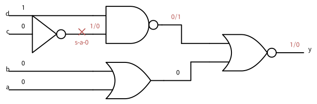
c = 0 excites the fault: the net is 1 in the good circuit and 0 in the faulty one (1/0). d = 1 lets the NAND gate pass the difference, and a = b = 0 let the NOR gate pass it. The test vector (a, b, c, d) = (0, 0, 0, 1) gives y = 1 in the good and y = 0 in the faulty circuit.
Exciting and propagating need controllability and observability: how easily a net can be set to a value from the inputs, and how easily its value can be seen at an output. Nets behind many levels of logic are hard to control and hard to observe. Justification fails when two required values conflict. The classic algorithms of automatic test pattern generation (ATPG) then go back and try other assignments, and when every alternative fails, the fault is untestable.
9.4.1 The D-Algorithm and PODEM
Roth’s D-algorithm (Roth 1966) made this search systematic in 1966, and its notation is still in use. It writes \(D\) for 1/0, a net that is 1 in the good and 0 in the faulty circuit, and \(\bar{D}\) for 0/1. It computes with five values: 0, 1, \(X\) for a value not assigned yet, \(D\), and \(\bar{D}\). A gate applies its function to the good and to the faulty value separately (Table 39). The non-controlling value at the other input lets \(D\) pass an AND gate, the controlling value blocks it. \(D\) and \(\bar{D}\) at the two inputs give a constant, because the good and the faulty circuit both see a 1 at one input and a 0 at the other.
| \(a\) | \(b\) | \(a\) AND \(b\) | \(a\) OR \(b\) | \(a\) XOR \(b\) |
|---|---|---|---|---|
| \(D\) | 0 | 0 | \(D\) | \(D\) |
| \(D\) | 1 | \(D\) | 1 | \(\bar{D}\) |
| \(D\) | \(X\) | \(X\) | \(X\) | \(X\) |
| \(D\) | \(D\) | \(D\) | \(D\) | 0 |
| \(D\) | \(\bar{D}\) | 0 | 1 | 1 |
The algorithm keeps two lists. The D-frontier holds the gates with \(D\) or \(\bar{D}\) at an input and \(X\) at the output, i.e., the gates through which the fault effect can still move on. The J-frontier holds the gates whose output value is required but not yet justified by their inputs. After each assignment, implication derives the values that follow directly from it, forward and backward, e.g., a 0 required at the output of an OR gate implies a 0 at each of its inputs. The algorithm proceeds in three steps:
- It excites the fault: the fault site gets \(D\) for a stuck-at-0 and \(\bar{D}\) for a stuck-at-1.
- It moves the fault effect on: it picks a gate of the D-frontier and sets its other inputs to the non-controlling value, or to any known value for an XOR gate, until \(D\) or \(\bar{D}\) reaches an output.
- It justifies the J-frontier: it picks input values for each gate in it, back to the primary inputs, the inputs of the design itself.
Where a step has several choices, e.g., which gate of the D-frontier, or which input of an OR gate justifies its 1, the algorithm records a decision. When two values conflict, or the D-frontier runs empty before the fault effect reaches an output, it goes back to the last decision and tries the next choice. When no choice is left, the fault is untestable.
In Figure 48, the stuck-at-0 at the inverter output gets \(D\), and \(c = 0\) follows by implication. The D-frontier holds the NAND gate, and \(d = 1\) propagates \(\bar{D}\) to its output. Now the D-frontier holds the NOR gate, and a 0 at its other input gives \(y = D\) at the output. The 0 required at the output of the OR gate implies \(a = b = 0\), so the J-frontier stays empty. No step had a second choice, and the test is \((a, b, c, d) = (0, 0, 0, 1)\). The J-frontier fills up when a required value has several justifications, e.g., a 0 at the output of an AND gate whose inputs are all unassigned, and then each choice is a decision.
The D-algorithm decides on internal nets, so it may find out only many steps later that a decision cannot be justified from the inputs. PODEM (Goel 1981) decides on the primary inputs only. It takes an objective, e.g., a 1 at the fault site, traces it back along a path to an input that has no value yet (the backtrace), assigns that input, and simulates the circuit forward. When the fault can no longer be excited, or no path of unassigned nets leads from the D-frontier to an output, it flips the last input decision, and when both values of that input have failed, it goes back to the decision before. Only the \(n\) inputs are decided, so the search tree has at most \(2^n\) leaves, and all values inside the circuit follow from the inputs by simulation, so they never conflict. Later ATPG algorithms refined this search.
9.4.2 SAT Solvers and Random Vectors
Modern tools often hand this search to a SAT solver, the same kind of solver as in the equivalence check of Section 5.8. A miter joins the good and the faulty netlist: both get the same inputs, an XOR compares each pair of outputs, and the solver searches for an input that sets one of the XORs to 1. Every solution is a test, and if there is none, the fault is proven untestable. The script sat_test.tcl does this with Yosys for one fault: it ties the listed cell pins to the stuck value in a copy of the netlist, builds the miter, and lets the command sat search:
atpg/sat_test.tcl
# SPDX-FileCopyrightText: 2026 Simon Dorrer
# SPDX-License-Identifier: Apache-2.0
# Description: Test generation for one stuck-at fault with a SAT
# solver. Builds a copy of the netlist with the fault, joins both in a
# miter, and searches an input for which the outputs differ. Usage:
#   TOP=cons PINS=u_or/C SA=0 yosys -c sat_test.tcl
# TOP is the module, read from $TOP.v unless NETLIST names the file.
# PINS lists the cell inputs that the fault forces to SA: one pin for
# a net with one load, all its loads for a net with several. (This
# misses a net that also drives an output port.)

yosys -import
set top $::env(TOP)
set netlist $top.v
if {[info exists ::env(NETLIST)]} { set netlist $::env(NETLIST) }
set lib $::env(PDK_ROOT)/ihp-sg13cmos5l/libs.ref/sg13cmos5l_stdcell
set lib $lib/lib/sg13cmos5l_stdcell_typ_1p20V_25C.lib

# The cell functions from the Liberty file, then the netlist
read_liberty -ignore_miss_func $lib
read_verilog $netlist
hierarchy -check -top $top

# The faulty copy: each listed pin is tied to the stuck-at value
copy $top faulty
yosys cd faulty
foreach p $::env(PINS) {
  lassign [split $p /] cell pin
  connect -port $cell $pin 1'b$::env(SA)
}
yosys cd ..

# The miter compares both copies, the solver searches a difference
miter -equiv -flatten -make_outputs $top faulty miter
hierarchy -top miter
tee -q -o sat.log sat -prove trigger 0 -show-inputs miter
set f [open sat.log]
set log [read $f]
close $f
if {[string match "*model found: FAIL*" $log]} {
  puts "TEST FOUND, the inputs (decimal):"
  set rows {^\s+\\in_(\S+)\s+(\d+)}
  foreach {- name value} [regexp -all -inline -line $rows $log] {
    puts "  $name = $value"
  }
} else {
  puts "NO TEST EXISTS: the fault is untestable"
}
Applying all input vectors would detect every detectable fault, but as in Section 4.6.2, their number explodes. The combinational 32-bit barrel shifter of Section 4 has 39 input bits, i.e., \(2^{39} \approx 5.5 \cdot 10^{11}\) vectors, which take 1.5 hours per die at 100 MHz. Fortunately, most faults are easy to detect, and a few random vectors find them. Fault simulation determines which faults a vector detects: it simulates the netlist with each fault injected and compares the outputs with those of the good netlist. ATPG tools therefore start with random vectors, drop the faults these detect, and search deterministically only for the rest. Some faults resist random vectors. The output of a 16-bit comparator with a constant is 1 for one of \(2^{16}\) input values, so 1000 random vectors detect its stuck-at-0 with a probability of only 1.5 %, and a probability of 99 % would take \(3.0 \cdot 10^5\) vectors. The deterministic search finds the single test at once. Finally, compaction removes vectors whose faults other vectors detect as well.
The IIC-OSIC-TOOLS image contains Fault (AUCOHL 2026) 0.9.4, an open-source DFT tool chain. fault atpg generates random vectors in batches, -v vectors at first and -r more in each further batch, simulates all faults with Icarus Verilog, and continues until it reaches the coverage that -m demands or the number of vectors that --ceiling allows. Then it compacts the vectors. It injects each fault with a force on a cell pin. Fault can also call deterministic ATPG programs, but none of them is available in the image, so here it relies on random vectors, and sat_test.tcl handles single faults.
TipExercise: Find the Test
All commands start in the folder content/dft/code/atpg, which holds the gate-level netlist cons.v of SG13CMOS5L cells.
Draw the circuit of
cons.vwith its cell instances and net names, and write down its function \(y = f(a, b, c)\) as a sum of products. Which product could you remove without changing the function?Find by hand a test for each of these faults:
abstuck-at-0,a_nstuck-at-1,bcstuck-at-1, andbcstuck-at-0. Write the values along the path with \(D\) and \(\bar{D}\), and note the D-frontier and the J-frontier at each step. Which values does each fault need to be excited and propagated? If you find no test, explain why none exists.Check your answers with the SAT solver. A fault on a net with one load needs only that load pin, e.g., for
abstuck-at-0:TOP=cons PINS=u_or/A SA=0 yosys -q -c sat_test.tclWhich pins does a stuck-at fault on the input
b_ineed? Is a stuck-at-0 at the pinAofu_bcalone testable?Let Fault generate a test set:
fault atpg cons.v -c $CELLS/sg13cmos5l_stdcell.v \
  -I $CELLS/sg13cmos5l_udp.v --clock clk_i --reset rst_ni \
  --activeLow -v 8 -m 100 --ceiling 32 -o cons.tv.json \
  --output-coverage-metadata cons.cov.yml
How many fault sites and faults does Fault find, and which coverage does it reach? Which faults stay undetected (the list
sa0Uncoveredincons.cov.yml, the listsa1Uncoveredof Fault 0.9.4 repeats it by mistake)? How many vectors remain after the compaction, which ones are they (cons.tv.json), and could fewer vectors detect the same faults? Does Fault agree with step 3 on the pinAofu_bc?Count the fault sites of
cons.vwith a site on each net and on each branch of a net with several loads, and ignore the unusedclk_iandrst_ni. How many stuck-at faults are there, and how many does the collapsing rule of Section 9.3 leave?python3 collapse.py cons.vsimulates every fault for all 8 inputs and groups the faults that give the same outputs. How many groups does it find, and why does it find fewer than the rule?
Before continuing, please finish the previous exercise. Once you are done, compare with the solution below.
TipSolution: Find the Test
- The circuit (Figure 49) computes \(y = ab + \bar{a}c + bc\). The product \(bc\) is the consensus of the other two and can be removed: for \(b = c = 1\), either \(a = 1\) and \(ab = 1\), or \(a = 0\) and \(\bar{a}c = 1\). So \(y = ab + \bar{a}c\).
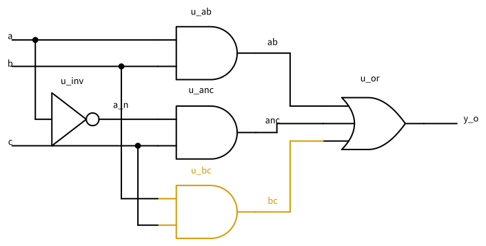
cons.v: \(y = ab + \bar{a}c + bc\). The term \(bc\) is the consensus of the other two: whenever \(b = c = 1\), either \(ab\) or \(\bar{a}c\) is 1 as well, so the gate u_bc never changes the output.
- With the inputs written as \((a, b, c)\):
abstuck-at-0: excite with \(a = b = 1\), soab= \(D\). The D-frontier holdsu_or, whose other inputsancandbcmust be 0:ancis 0 becausea_nis 0, and with \(b = 1\),bc= 0 implies \(c = 0\). Then \(y = D\), and the test is (1, 1, 0), with \(y\) = 1 in the good and 0 in the faulty circuit.a_nstuck-at-1: excite witha_n= 0, i.e., \(a = 1\), soa_n= \(\bar{D}\). The D-frontier holdsu_anc, and \(c = 1\) givesanc= \(\bar{D}\). Then it holdsu_or, andab= 0, i.e., \(b = 0\), which also keepsbcat 0, gives \(y = \bar{D}\). The test is (1, 0, 1).bcstuck-at-1:bc= \(\bar{D}\) needsbc= 0 in the good circuit. The D-frontier holdsu_or, andab=anc= 0 propagate \(\bar{D}\) to \(y\). Each of the three AND gates now needs a 0 at its output that two inputs could give, so all three sit in the J-frontier, and one decision, e.g., \(a = 0\) and \(c = 0\), justifies all of them. Any input with \(y\) = 0 in the good circuit is a test: (0, 0, 0), (0, 1, 0), (1, 0, 0), or (1, 0, 1).bcstuck-at-0: excite with \(b = c = 1\), sobc= \(D\). The D-frontier holds onlyu_or, which needsab= 0 andanc= 0. With \(b = 1\),ab= 0 implies \(a = 0\), and with \(c = 1\),anc= 0 impliesa_n= 0, i.e., \(a = 1\). The implications conflict, and no step had another choice, so no test exists: the fault is untestable, becausebcis redundant.
- The solver confirms all four: it prints (1, 1, 0) for
PINS=u_or/A SA=0, (1, 0, 1) forPINS=u_anc/A SA=1, (0, 0, 0) forPINS=u_or/C SA=1, and “NO TEST EXISTS” forPINS=u_or/C SA=0. A fault onb_iacts on both cells it drives, so it needsPINS="u_ab/B u_bc/A". The solver finds (1, 1, 1) for stuck-at-0 and (1, 0, 0) for stuck-at-1. A stuck-at-0 at the pinAofu_bcalone forcesbcto 0, likebcstuck-at-0, and is untestable as well. - Fault finds 19 fault sites, the 15 cell pins and the 4 ports
a_i,b_i,c_i, andy_o(it leaves outclk_iandrst_ni), i.e., 38 faults, and reaches 94.74 %, 36 of 38. The two undetected faults, the stuck-at-0 atu_bc.Xand atu_or.C, are both the untestable stuck-at-0 on the netbc. The compaction keeps 4 vectors: (0, 0, 1), (1, 0, 1), (0, 1, 0), and (1, 1, 0). Fewer cannot detect the same faults:abstuck-at-0 has the single test (1, 1, 0), because in (1, 1, 1)bc= 1 hides the fault.ancstuck-at-0 has the single test (0, 0, 1), anda_nstuck-at-1 the single test (1, 0, 1). The inputc_istuck-at-1 needs \(a = c = 0\), which none of these three vectors has. Fault reports the stuck-at-0 at the pinAofu_bcas detected, which step 3 proved untestable. Fault forces the pin, and Icarus merges the input pin of a cell with the net it connects to when the net has one bit. The force thus acts on the whole netb_i, its stem, instead of its branch tou_bcalone, so the fault that Fault simulates isb_istuck-at-0, which (1, 1, 0) detects. Commercial ATPG tools list the stem and every branch of a net as separate faults. - The 8 nets
a_i,b_i,c_i,a_n,ab,anc,bc, andy_oand the two branches of each input give 14 sites and 28 faults. With \(P_O = 1\), \(F_O = 3\), \(G_I = 1 + 3 \cdot 2 + 3 = 10\), and \(N_I = 1\), the rule leaves \(2 \cdot (1 + 3) + 10 - 1 = 17\) faults.collapse.pyfinds 13 groups, one of them the untestablebc,u_bc.A, andu_bc.Bstuck-at-0. The rule merges only faults that are equivalent within one gate. The four extra merges all involveu_bc, the gate of the redundant product, whose faults the rest of the function absorbs.u_bc.Astuck-at-1 makesbc= \(c\), so \(y = ab + c\), the same function as witha_nstuck-at-1.b_istuck-at-1 gives \(y = a + c\), whether or not its branch intou_bcsees the fault, so it equalsu_ab.Bstuck-at-1. Fault counts differently: it lists every cell pin and port bit, so a net with one load has two sites, its driver pin and its load pin, which are equivalent.
9.5 Scan Design
In a sequential circuit, the logic between the registers is reachable only through the registers. To test a gate inside a state machine, a test must first steer the machine into a state that excites the fault, and then wait until the difference reaches an output, over many clock cycles. Sequential ATPG exists, but it is slow, and in large designs, its coverage stays low.
Scan design makes every flip-flop controllable and observable. Each flip-flop becomes a scan flip-flop, with a multiplexer in front of its input (Figure 50). With the scan enable low, it loads its functional input. With the scan enable high, it loads the output of the previous flip-flop in the chain, and all scan flip-flops together form a shift register, the scan chain, from an input pin scan_in to an output pin scan_out. The tester can now shift any state into the flip-flops, and shift out any state they captured. For the test generation, the output Q of each flip-flop becomes an input of the logic, and its input D an output, so the sequential problem turns into the combinational one of Section 9.4.
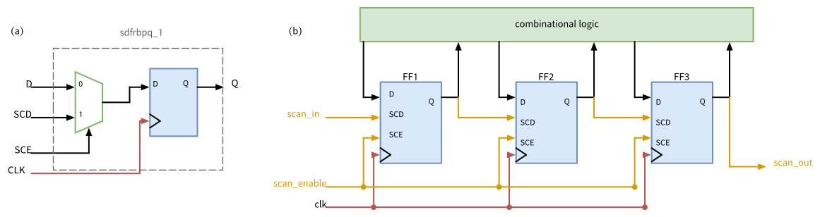
sdfrbpq_1 is a flip-flop with a multiplexer in front: with SCE = 0, it loads the functional input D, with SCE = 1 the scan input SCD. (b) The scan flip-flops of a design form a shift register, the scan chain (orange), from scan_in through every flip-flop to scan_out. One scan_enable switches all of them between shifting and normal operation.
SG13CMOS5L has five scan flip-flops (Section 5.3): sdfrbpq_1 and sdfrbpq_2 with the output Q, sdfrbp_1 and sdfrbp_2 with Q and Q_N, and sdfbbp_1 with set and reset. Their scan input is SCD, their scan enable SCE. sdfrbpq_1 takes 63.5 µm², 30 % more than dfrbpq_1 with 49.0 µm², but less than dfrbpq_1 and mux2_1 together (67.1 µm²). The Liberty file describes the scan function of each cell in a test_cell group, from which tools learn which pin is the scan input and which flip-flop it can replace.
Figure 51 shows how the tester applies the patterns one after the other. A scan pattern is a test vector arranged for the scan test: the values of the flip-flops in the order in which they are shifted in, and the values of the primary inputs. While scan_enable is high, every clock edge shifts the chain by one bit, so after \(L\) edges, a chain of \(L\) flip-flops holds the pattern. The tester applies the primary inputs, compares the primary outputs, sets scan_enable low, and gives one clock edge, the capture, at which every flip-flop loads the response of the logic. The next \(L\) shift edges unload this response at scan_out while they load the next pattern, and the tester compares each bit with its expected value. Before the first pattern, a test program runs a chain test: it shifts a known sequence such as 0011… through the chain without a capture and checks that it arrives unchanged at scan_out.
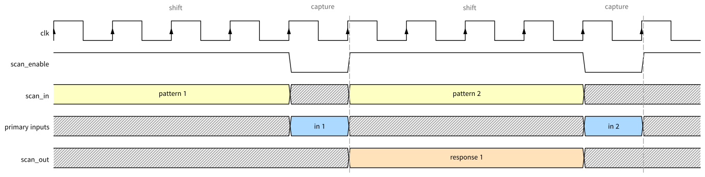
scan_enable is high, every rising clock edge shifts the chain by one position, so four edges load pattern 1 from scan_in. In the capture cycle, scan_enable is low, and the edge at its end (dashed) captures the response of the logic to the pattern and to the primary inputs. The next four shift edges unload the response at scan_out and load pattern 2 at the same time.
For \(N\) patterns and a chain of \(L\) flip-flops, the test takes \((N + 1) L + N\) clock cycles: \(N + 1\) shift phases of \(L\) cycles, because the last response must come out as well, and \(N\) captures. The shifts dominate, so designs split their flip-flops into several chains that shift in parallel, each with its own pins. When the pins run out, on-chip test compression feeds hundreds of short chains from a few pins through a decompressor and compacts their outputs. The shift clock is often slower than the functional clock, because shifting random patterns toggles many more flip-flops at once than normal operation, which draws a high current.
In the open-source flow, OpenROAD (The OpenROAD Project 2026) inserts the chains. scan_replace replaces every flip-flop by a scan flip-flop with the same function, and execute_dft_plan stitches the chains and adds the ports scan_enable_0, scan_in_0, scan_out_0, and so on. In a complete flow, scan_replace runs before the placement, because it changes the cell areas, and execute_dft_plan after it, so that each chain connects neighbors on the die. The script dft.tcl runs both on a netlist without placement:
scan/dft.tcl
# SPDX-FileCopyrightText: 2026 Simon Dorrer
# SPDX-License-Identifier: Apache-2.0
# Description: Scan insertion with OpenROAD. Replaces every flip-flop
# by its scan version and stitches the scan chains. Usage, in the
# folder of the netlist: TOP=bs_reg openroad -no_init -exit dft.tcl
# (reads $TOP.nl.v, writes ${TOP}_scan.nl.v). CLOCKS lists the clock
# inputs (default clk_i), MAX_LENGTH limits the length of a chain
# (default 100).

set top $::env(TOP)
set clocks clk_i
if {[info exists ::env(CLOCKS)]} { set clocks $::env(CLOCKS) }
set max_length 100
if {[info exists ::env(MAX_LENGTH)]} {
  set max_length $::env(MAX_LENGTH)
}

set lib $::env(PDK_ROOT)/ihp-sg13cmos5l/libs.ref/sg13cmos5l_stdcell
read_lef $lib/lef/sg13cmos5l_tech.lef
read_lef $lib/lef/sg13cmos5l_stdcell.lef
read_liberty $lib/lib/sg13cmos5l_stdcell_typ_1p20V_25C.lib
read_verilog $top.nl.v
link_design $top

# The chains are built per clock, so the clocks must be known
foreach clk $clocks {
  create_clock -name $clk -period 100 [get_ports $clk]
}
set_dft_config -max_length $max_length -clock_mixing no_mix

# Replace the flip-flops, plan the chains, and stitch them
scan_replace
report_dft_plan -verbose
execute_dft_plan
write_verilog ${top}_scan.nl.v
LibreLane, the flow of Section 10, has no step for scan insertion. For the test generation, fault cut turns each flip-flop into an input and an output, and fault atpg generates vectors for the result. The file scl.yml tells Fault which cells are flip-flops. The following commands synthesize the barrel shifter between two registers of Section 6.7 with 8 bits instead of 32, cut its flip-flops open, and generate vectors:
cd /foss/designs/vlsi-design/content/dft/code/scan
yosys -p "read_verilog -sv \
  ../../../verification/code/barrel_shift/rtl/barrel_shift.sv \
  ../../../sequential/code/bs_reg/rtl/bs_reg.sv; \
  chparam -set WIDTH 8 bs_reg; synth -top bs_reg; flatten; \
  dfflibmap -liberty $LIB; abc -constr $CONSTR -liberty $LIB; \
  opt_clean; stat -liberty $LIB; write_verilog -noattr bs_reg.nl.v"
fault cut bs_reg.nl.v --sclConfig scl.yml --clock clk_i \
  --reset rst_ni --activeLow -o bs_reg.cut.v
fault atpg bs_reg.cut.v -c $CELLS/sg13cmos5l_stdcell.v \
  -I $CELLS/sg13cmos5l_udp.v --clock clk_i --reset rst_ni \
  --activeLow -v 100 -r 100 -m 100 --ceiling 1000 \
  -o bs_reg.tv.json
Fault holds the reset inactive and finds 580 fault sites, i.e., 1160 faults. Figure 52 shows how the coverage grows with the number of random vectors: 97.84 % after 100 vectors and 99.66 % from 350 on. The four faults that remain are not missed by chance: sat_test.tcl proves each of them untestable, because ABC left redundant logic in the netlist. In the fault model of Fault, the test coverage is therefore 100 %. After 1000 vectors, Fault stops at its ceiling and compacts the set to 32 vectors that detect the same 1156 faults.
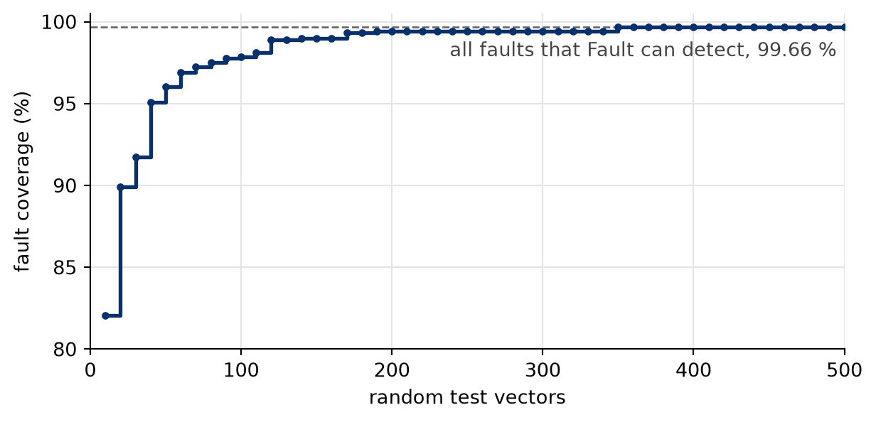
bs_reg, with its flip-flops cut into inputs and outputs, simulated by Fault with -v 10 -r 10, i.e., in batches of 10 vectors. Most faults are detected within the first 50 vectors. From 350 vectors on, all 1156 faults that the fault model of Fault can detect are found. The other 4 of the 1160 faults are untestable, so the coverage stays at 99.66 %.
Coverage numbers depend on the fault model. Fault injects a fault with a force on a cell pin. Icarus merges the input pin of a cell with the net it connects to when the net has one bit, so the force acts on the whole net, its stem. A force on a pin at one bit of a vector acts on that pin alone, the branch of the net to this cell. In this netlist, 300 of the 379 inputs of the logic cells sit on nets of one bit, so Fault mostly simulates faults on whole nets, where commercial ATPG tools list the stem and every branch as separate faults. In a fault simulation with a wire of its own for every cell input, the 32 vectors miss 59 of the 1034 faults at the pins of the 138 logic cells. The SAT solver proves 12 of them untestable, and the other 47 would need more vectors, so the test coverage at the cell pins is 95.4 %.
The scan flip-flop also costs speed. On the worst path of the 8-bit bs_reg between two registers, its setup time is 0.204 ns instead of 0.125 ns for dfrbpq_1, and its clock-to-output delay 0.344 ns instead of 0.309 ns. The gates on the path take 0.019 ns longer, mainly because the last of them drives the larger input D of the scan flip-flop. The minimum period rises from 1.30 to 1.43 ns.
Figure 53 summarizes the steps from the synthesized netlist to the patterns for the tester, with the tools of this chapter. The conversion into scan patterns and their simulation follow in the next exercise, the equivalence check after it.
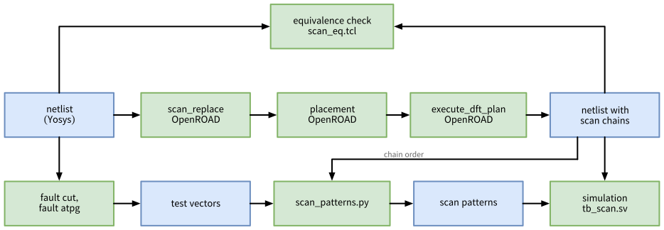
scan_replace turns the flip-flops into scan flip-flops before the placement, and execute_dft_plan stitches the chains after it. The layout flow then continues with the clock tree and the routing. Fault generates test vectors on the netlist with its flip-flops cut open, scan_patterns.py arranges them along the chain into scan patterns, and tb_scan.sv applies these to the netlist with the scan chains in a simulation. scan_eq.tcl checks that the scan insertion did not change the function.
TipExercise: Insert a Scan Chain
All commands start in the folder content/dft/code/scan and use bs_reg.nl.v and bs_reg.tv.json from the commands above.
Sketch the registers of the 8-bit
bs_regwith their widths and draw a scan chain through all of their flip-flops. How long is the chain?Insert the chain with
TOP=bs_reg openroad -no_init -exit dft.tcl. In which order does OpenROAD chain the registers, and which flip-flop drivesscan_out_0? Compare the area ofbs_reg.nl.vandbs_reg_scan.nl.v:yosys -p "read_liberty -lib $LIB; read_verilog bs_reg_scan.nl.v; \ stat -liberty $LIB"How much area does the scan insertion add in total and in percent, and which cells changed?
Convert the vectors of Fault into scan patterns and run the scan test of
tb/tb_scan.sv:python3 scan_patterns.py bs_reg_scan.nl.v bs_reg.tv.json > bs_reg.pat iverilog -g2012 -gno-specify -DPATTERNS=\"bs_reg.pat\" -o scan.vvp \ $CELLS/sg13cmos5l_udp.v $CELLS/sg13cmos5l_stdcell.v \ bs_reg_scan.nl.v tb/tb_scan.sv vvp -n scan.vvpWhat do the chain test and the scan test report? Where do the expected responses come from?
Inject a defect: compile again with
-DFAULT=_007_ -DSA=0added, then with-DFAULT=_008_ -DSA=1. Which defect does the scan test detect, and why not the other one? Repeat both with random patterns, i.e., without-DPATTERNS=.... What changes, and why?The tester shifts at 10 MHz. How long does the scan test of the 32 patterns take with one chain? Build three chains of at most 7 flip-flops instead with
MAX_LENGTH=7 TOP=bs_reg openroad -no_init -exit dft.tcl(it overwritesbs_reg_scan.nl.v). How long does the test take then?
Before continuing, please finish the previous exercise. Once you are done, compare with the solution below.
TipSolution: Insert a Scan Chain
bs_reghas the registersdata_q(8 bits),shamt_q(3 bits),mode_q(2 bits), andout_q(8 bits), so the chain has 21 flip-flops (Figure 54).
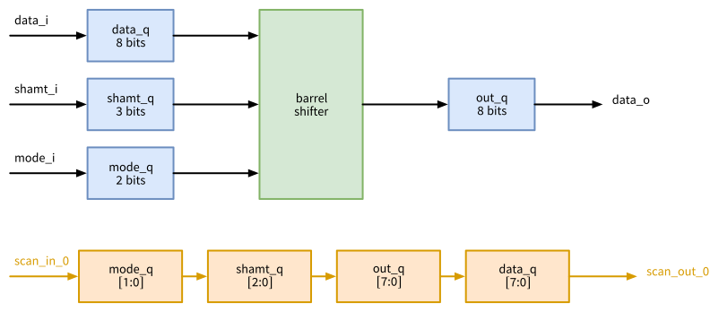
bs_reg after scan insertion. Top: its registers in normal operation. Bottom: the same 21 flip-flops as one scan chain (orange), from scan_in_0 through mode_q, shamt_q, out_q, and data_q, each from its highest bit to its lowest, to scan_out_0, the output of data_q[0]. scan_enable_0 drives all 21 SCE pins (not drawn).
- Without a placement, OpenROAD has no wire lengths to minimize, and here it chains the flip-flops in descending order of their instance names, from
_288_atscan_in_0to_268_atscan_out_0:mode_q,shamt_q,out_q, anddata_q, each from its highest bit to its lowest.scan_out_0is connected directly todata_q[0], the output of_268_, and eachSCDto the output of the previous flip-flop, without any additional cell. The area grows from 2543.45 to 2848.27 µm², by 304.82 µm² or 12.0 %, and only the flip-flops changed: each of the 21 became ansdfrbpq_1, 14.52 µm² larger thandfrbpq_1. scan_patterns.pyfollows the chain fromscan_in_0and reports its 21 flip-flops. The chain test reports 0 of 21 bits wrong, and the scan test 32 patterns with 0 bits that differ. The expected responses come from the second instancegoldof the same netlist, which is fault-free and receives the same patterns, just as a test program takes its expected values from a simulation of the fault-free netlist. The file of Fault also holds the fault-free response of each vector (goldenOutput), but the testbench does not use it.- With
_007_stuck-at-0, one bit differs, so the scan test detects it._008_stuck-at-1 stays undetected:_008_is the output of_253_and drives only the inputA2of_254_, and its stuck-at-1 is one of the four untestable faults, together with both faults at the inputBof_253_and the stuck-at-1 atA2of_254_. With 32 random patterns,_007_stuck-at-0 stays undetected too, and no bit differs: none of the random patterns excites the fault and propagates it to a flip-flop. Fault selected its 32 vectors from 1000 random ones, so that together they detect every fault that it could detect. - One chain: \((32 + 1) \cdot 21 + 32 = 725\) cycles, i.e., 72.5 µs at 10 MHz. Three chains of 7 flip-flops: \((32 + 1) \cdot 7 + 32 = 263\) cycles, i.e., 26.3 µs.
Scan insertion changes the netlist, so the equivalence check of Section 5.8 runs after it. With the scan inputs tied to 0, the scanned netlist must compute exactly what the netlist before scan insertion computed. The script scan_eq.tcl checks this with the Yosys commands equiv_make, equiv_simple, and equiv_induct. They match the nets of both netlists by name, among them the outputs of all flip-flops, and prove each matched pair, a point of the check, equal. After the exercise, bs_reg_scan.nl.v holds the netlist with three chains, and TOP=bs_reg yosys -q -c scan_eq.tcl in the folder scan proves all 163 points of bs_reg equal, as it does for the netlist with one chain. With the scan inputs tied to 1 (TIE=1), the check fails: 32 points of the netlist with three chains and 38 of the one with one chain cannot be proven equal.
Without a placement, dft.tcl chains the flip-flops in an order that ignores their positions on the die. The script dft_place.tcl runs the complete sequence on the 32-bit bs_reg with its 71 flip-flops: scan_replace, a floorplan with 50 % utilization, the placement, and then execute_dft_plan, which now orders the chain along the placement. In the folder scan:
yosys -p "read_verilog -sv \
  ../../../verification/code/barrel_shift/rtl/barrel_shift.sv \
  ../../../sequential/code/bs_reg/rtl/bs_reg.sv; \
  synth -top bs_reg; flatten; dfflibmap -liberty $LIB; \
  abc -constr $CONSTR -liberty $LIB; opt_clean; \
  write_verilog -noattr bs_reg32.nl.v"
NETLIST=bs_reg32.nl.v TOP=bs_reg \
  openroad -no_init -exit dft_place.tcl
The chain now connects neighbors: on the same placement, the distances between neighbors in the chain add up to 911 µm, against 3024 µm for the same flip-flops in the order without placement, 70 % less (Figure 55). The scan flip-flops of SG13CMOS5L have no separate scan output, so the chain wire hangs on the output Q of each flip-flop, which also drives the logic. A short chain therefore saves routing tracks, and delay and power in normal operation as well as during the shift. OpenROAD also has the command scan_opt for reordering the chains of a placed design, but in this version, it only warns that it is not implemented yet.
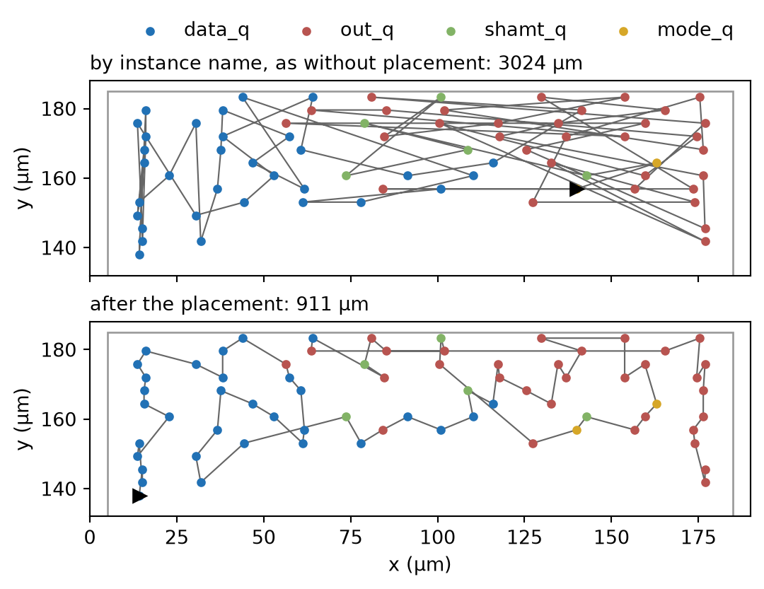
bs_reg with 71 flip-flops, placed and stitched by dft_place.tcl. Each dot is a scan flip-flop, colored by its register, the gray line is the chain, and the triangle marks the first flip-flop, at scan_in_0. Top: the same flip-flops in the order of a chain stitched without placement, by descending instance name, 3024 µm of wire. Bottom: the order of execute_dft_plan after the placement, 911 µm. Each length adds the distances between the centers of neighbors in the chain, horizontally plus vertically. The plot shows only the upper part of the 180 µm wide core, where the placement put all flip-flops.
9.6 Design Rules for Testability
Scan works only if the tester controls the design in test mode. Every flip-flop must shift and capture at the clock of the tester, nothing may disturb the chain while it shifts, and the logic must give values that the ATPG can predict. ATPG tools check rules for this before they generate any pattern. The most important rules:
- Every clock comes from a pin. In test mode, the tester drives all clocks. A clock from a divider (Section 3.4.2), from a phase-locked loop (PLL), or from another flip-flop (Section 6.8) needs a multiplexer that selects a clock pin in test mode. A clock enable, which replaces the divider in Section 3.4.2, needs nothing. At-speed tests take faster pulses from an on-chip PLL, through a clock controller that the tester controls (Section 9.7).
- Every clock gate has a test enable. An integrated clock gate (Section 7.7) switches off the clock while its enable is low, and the enable comes from logic whose flip-flops are shifting, so the gated flip-flops would miss shift edges. The clock gate
slgcp_1(30.8 µm², against 27.2 µm² forlgcp_1) therefore has the inputSCE. The cell ORsSCEwithGATEin front of the latch (latch_posedge_precontrol), and the Liberty file marksSCEasclock_gate_test_pin. Connected to the scan enable, it turns on every gated clock while the chain shifts. Clock gating is thus fine for scan, as long as the test enable is connected. Neither Yosys nor OpenROAD connects it to the scan enable. Forcg_regof Section 7.7 withWIDTH= 8,clockgateconnects onlyGATE,CLK, andGCLKofslgcp_1, or tiesSCEto 0 with-tie_lo SCE. OpenROAD puts the 8 gated flip-flops into a chain, warns that the clock gate is not a scan cell, and leavesSCEunconnected. - Asynchronous resets are controlled from a pin. The tester holds a reset from a pin inactive during the whole test. A reset that the design generates itself, e.g., in a power-on-reset circuit, in the reset synchronizer of Section 8.8, or from another flip-flop, needs special care in test mode. The following exercise shows why.
- No latches, no combinational loops, no pulse generators. A latch passes or holds depending on its gate, so it is neither a clean input nor a clean output for the ATPG. Latches are made transparent in test mode, or the design uses flip-flops only (Section 6.11). The latch inside a clock gate is the exception, because its test enable controls it. A combinational loop has no defined value and is broken in test mode. A pulse generator built from a delay chain, e.g., an XOR of a signal and its delayed copy, gives pulses whose width depends on the process, which scan cannot test.
- No unknown values reach a flip-flop. Memories (Section 3.4.3), analog blocks, and black boxes give values that the ATPG cannot predict (
x), and anxcaptured in a flip-flop makes its bit of the response useless. A tri-state bus (Section 3.4.4) floats or has two active drivers when a shifted state enables none or two of them. Such blocks get a bypass or a wrapper of scan flip-flops in test mode, and memories a test of their own (Section 9.7). - One chain per clock domain. Flip-flops of different clocks see their edges at different moments, so a chain should not mix them. With
-clock_mixing no_mix, OpenROAD builds one chain per clock. For the asynchronous FIFO of Section 8.6, it builds a chain of 43 flip-flops atwclk_iand one of 11 atrclk_i, which sharescan_enable_0. A chain that crosses from one clock to another needs a lockup latch at the crossing, a latch on the launching clock that is transparent while this clock is low. It delays the data by half a period, so that a skew of up to about half a period between the clocks cannot cause a hold violation. During the capture, the paths between asynchronous clocks are not timed (Section 8.7), so their results are unknown when both clocks pulse. The ATPG then captures one clock domain at a time, or ignores the flip-flops behind such paths, e.g., the first stage of each synchronizer. - The chain is a timing path, too. The connection from
Qto theSCDof the next flip-flop has no logic, so it is among the shortest paths of a design and the first to fail the hold check when the clock reaches the next flip-flop late (Section 6.10). In the scanned 8-bitbs_reg, the 20 paths with the smallest hold slack all end at anSCDpin, from 0.292 ns with an ideal clock, which already includes the clock uncertainty of 0.1 ns, while the functional paths start at 0.383 ns. A clock skew of 0.3 ns between two neighbors in the chain would violate the hold check, and from about 0.39 ns, the chain itself would fail. After the clock tree synthesis, the layout flow fixes hold violations on the scan paths like on any other path, with delay cells.scan_enable_0drives all 21SCEpins, a net with a high fanout like a reset, which must settle within one shift cycle.
TipExercise: Make It Testable
All commands start in the folder content/dft/code/reset. It holds the reference solution rtl/bs_reg_rs_tm.sv, so move it out of the way first: cd /foss/designs/vlsi-design/content/dft/code/reset, then mv rtl/bs_reg_rs_tm.sv bs_reg_rs_tm_solution.sv.
The module
bs_reg_rsof Section 8.8 puts a reset synchronizer in front ofbs_reg. Sketch it: the two flip-flops of the synchronizer, the reset net to the registers ofbs_reg, and a scan chain through all flip-flops. What does the output of the second synchronizer flip-flop drive?Synthesize
bs_reg_rswith 8 bits, insert a scan chain, and run the scan test:yosys -p "read_verilog -sv \ ../../../verification/code/barrel_shift/rtl/barrel_shift.sv \ ../../../sequential/code/bs_reg/rtl/bs_reg.sv \ ../../../cdc/code/reset/rtl/rst_sync.sv \ ../../../cdc/code/reset/rtl/bs_reg_rs.sv; \ chparam -set WIDTH 8 bs_reg_rs; synth -top bs_reg_rs; flatten; \ dfflibmap -liberty $LIB; abc -constr $CONSTR -liberty $LIB; \ opt_clean; stat -liberty $LIB; \ write_verilog -noattr bs_reg_rs.nl.v" TOP=bs_reg_rs openroad -no_init -exit ../scan/dft.tcl iverilog -g2012 -gno-specify -DTOP=bs_reg_rs -DLEN=23 -o scan.vvp \ $CELLS/sg13cmos5l_udp.v $CELLS/sg13cmos5l_stdcell.v \ bs_reg_rs_scan.nl.v ../scan/tb/tb_scan.sv vvp -n scan.vvpHow long is the chain, and what do the chain test and the scan test report?
What happens to the other flip-flops of the chain while a 0 passes through the second synchronizer flip-flop? Why does the scan test not notice anything?
Draw a fix. The registers of
bs_regmust take their reset from the synchronizer in normal operation and from the pinrst_niduring the test. A new inputtest_mode_i, which the tester holds at 1 during the whole test, selects between both.Write
rtl/bs_reg_rs_tm.svwith the modulebs_reg_rs_tm. Synthesize it as in step 2, withrtl/bs_reg_rs_tm.svadded to the files,bs_reg_rs_tminstead ofbs_reg_rs, and the netlistbs_reg_rs_tm.nl.v. Insert the chain withTOP=bs_reg_rs_tmand run the testbench with-DTOP=bs_reg_rs_tm -DLEN=23 -DTEST_MODE. What does the chain test report now? What does the fix cost, and which part of the design does the test no longer reach?
Before continuing, please finish the previous exercise. Once you are done, compare with the solution below.
TipSolution: Make It Testable
- The second flip-flop of the synchronizer,
rst_no, drives the reset inputs of all 21 flip-flops ofbs_reg. A scan chain through all flip-flops passes through both synchronizer flip-flops,meta_qandrst_no. - The chain has 23 flip-flops. The chain test reports 11 of 23 bits wrong, the scan test 32 patterns with 0 bits that differ.
- Whenever a 0 shifts into the flip-flop
rst_no, its output resets all 21 flip-flops ofbs_regat once, and the bits they hold are lost. The scan test compares with a copy of the same netlist, which loses its bits in the same way, so all responses agree and the error stays hidden. With the expected values that an ATPG tool computes for an intact chain, the scan test would fail on every die, good or defective. Either way, the patterns are useless. This is why a test program starts with the chain test, and why ATPG tools check the reset rule before they generate patterns. - A multiplexer in front of the reset of the registers (Figure 56):
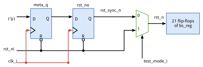
test_mode_i = 0), the registers get the synchronized reset rst_sync_n. In test mode, the multiplexer passes rst_ni from the pin, so the tester holds the reset inactive while the chain shifts, whatever the two synchronizer flip-flops in the chain contain.
- The reference solution:
reset/rtl/bs_reg_rs_tm.sv
// SPDX-FileCopyrightText: 2026 Simon Dorrer
// SPDX-License-Identifier: Apache-2.0
// Description: The barrel shifter between two registers behind a
// reset synchronizer (bs_reg_rs), with a test mode: during the scan
// test, the registers take their reset directly from the pin rst_ni.

`default_nettype none

module bs_reg_rs_tm #(
  parameter int unsigned WIDTH = 32  // power of two
) (
  input  logic                     clk_i,
  input  logic                     rst_ni,
  input  logic                     test_mode_i,  // 1 during the test
  input  logic [WIDTH-1:0]         data_i,
  input  logic [$clog2(WIDTH)-1:0] shamt_i,
  input  logic [1:0]               mode_i,
  output logic [WIDTH-1:0]         data_o
);

  logic rst_sync_n, rst_n;

  rst_sync u_rst_sync (
    .clk_i (clk_i),
    .rst_ni(rst_ni),
    .rst_no(rst_sync_n)
  );

  // In test mode, the tester controls the reset of the registers
  assign rst_n = test_mode_i ? rst_ni : rst_sync_n;

  bs_reg #(.WIDTH(WIDTH)) u_bs_reg (
    .clk_i  (clk_i),
    .rst_ni (rst_n),
    .data_i (data_i),
    .shamt_i(shamt_i),
    .mode_i (mode_i),
    .data_o (data_o)
  );

endmodule

`default_nettype wire
The chain test now reports 0 of 23 bits wrong. The fix costs one mux2_1 (18.1 µm²) in front of the 21 reset pins and one input. The total area changes by only 1.8 µm², from 2661.5 to 2663.3 µm², because ABC maps the barrel shifter slightly differently. In test mode, the multiplexer never selects rst_sync_n, so the path from the synchronizer to the registers is not tested. The two synchronizer flip-flops are still in the chain, and their inputs are tested at the capture.
9.7 Beyond Scan
Scan with stuck-at patterns is the backbone of the test of digital logic, but a complete test program contains more:
- At-speed test. Stuck-at patterns can be shifted and captured slowly. A transition fault needs a launch and a capture exactly one functional clock period apart. In launch on capture (LOC), two capture pulses at the functional frequency follow the shift: the first launches the transition, the second captures it. In launch on shift (LOS), the last shift edge launches the transition, so
scan_enablemust fall within one functional period before the capture edge. The fast pulses come from the on-chip PLL, through a clock controller that the tester triggers. - Built-in self-test (BIST). A linear feedback shift register (LFSR) on the chip generates pseudo-random patterns, and a multiple-input signature register (MISR) compacts the responses into a signature, which is compared with the signature of the fault-free design at the end. The tester only starts the test and reads the result, which also works in the field, e.g., at every start of a car. A wrong response gives the fault-free signature, which is called aliasing, with a probability of only about \(2^{-n}\) for an \(n\)-bit MISR. Memories get a memory BIST: a controller writes and reads march patterns, sequences of writes and reads that walk up and down the addresses, and finds cells that are stuck, that disturb their neighbors, or that lose their data. The SRAM macros of SG13CMOS5L (Section 3.4.3) need such a controller, and a bypass, so that scan can test the logic around them.
- Boundary scan (JTAG). The standard IEEE 1149.1 puts a scan cell at every pin of a chip and connects them into a chain, which the test access port (TAP) with the pins
TCK,TMS,TDI,TDO, and optionallyTRSTcontrols. On a board, it tests the solder joints and the wires between the chips without probing them. The same port gives access to internal scan chains and to debug logic, e.g., of a processor.fault tapadds a TAP controller to a netlist with a scan chain. - Parametric tests and binning. Besides the logic, the test measures the quiescent current, the input thresholds and output drivers of the pads, and the maximum clock frequency, by which parts can be sorted into speed grades.
- Diagnosis. When a die fails, its failing patterns and bits point to the faults that explain them, and the analysis of many failing dies shows the fab where its process creates defects.
NoteDifetto
Difetto, a complete rewrite of Fault, adds scan insertion and test generation to LibreLane as a plugin. It is still at an early stage, it is not in the IIC-OSIC-TOOLS image, and it has no scan cell mapping for SG13CMOS5L yet, so this course stays with OpenROAD and Fault. We may use it in the next edition of this course.
9.8 Summary
- Every manufactured die is tested, on the wafer and after packaging. Random defects cause the catastrophic, process variations the parametric yield loss, and a burn-in removes weak parts before they fail early in the field. The defect level \(1 - Y^{1-T}\) of the shipped parts depends on the yield and the fault coverage: 99 % coverage at 80 % yield leaves one defective part in 449.
- The single stuck-at fault model fixes one net, branch, or pin at 0 or 1, and fault collapsing merges equivalent faults. Transition, path delay, bridging, stuck-open, and stuck-on faults and IDDQ testing cover other defects. A transition test detects an extra delay only if it exceeds the slack of the tested path. A stuck-on transistor can hide from every static logic test and show only in IDDQ. Untestable faults sit in redundant logic. The test coverage leaves them out.
- A test excites a fault, propagates the difference, \(D\) or \(\bar{D}\), to an output, and justifies the required values from the inputs. The D-algorithm and PODEM search these values and go back on a conflict. ATPG tools start with random vectors and fault simulation and solve the rest with a deterministic search, today often with a SAT solver on a miter of the good and the faulty netlist.
- Scan replaces every flip-flop by a scan flip-flop and connects them into chains. Shift, capture, and shift turn the test of a sequential circuit into a combinational one. A test of \(N\) patterns over chains of \(L\) flip-flops takes \((N + 1) L + N\) cycles. In the 8-bit
bs_reg, scan insertion adds 12 % area. The 32 vectors of Fault detect every fault that its model can detect, but only 95.4 % of the detectable faults at the cell pins: coverage depends on the fault model. Stitched after the placement, the chain of the 32-bitbs_reggets 70 % shorter. - Scan needs clocks and resets from pins, clock gates with a connected test enable, no latches, loops, or unknown values, one chain per clock domain, and hold-safe scan paths. A reset synchronizer needs a test-mode bypass, or the chain breaks while it shifts.
- At-speed test, BIST for logic and memories, and boundary scan complete the test of a chip.
In Section 10, LibreLane takes the netlist through placement, clock tree synthesis, and routing to the layout. It inserts no scan chains, but the hold fixing and the equivalence check of this chapter return there.
10 The RTL-to-GDSII Flow with LibreLane
The netlists of the previous chapters exist only as text. To become a chip, every cell needs a place on the die, every net a wire in metal, and every clock a tree of buffers. The result must then pass the timing checks again, now with real wires, and checks that only a layout can fail: the design rules of the process and the comparison of the layout with the netlist. This chapter takes the barrel shifter between two registers of Section 6.7 through LibreLane (LibreLane Project 2026), the open-source RTL-to-GDSII flow of this course, from its RTL to a GDSII layout, one step at a time. It ends with the chip top level of the AMS chip template (Section 1.10), which puts such blocks into a padframe.
Note
All code of this chapter is available in the folder content/digital_flow/code of the course repository: the LibreLane configuration, the equivalence check, and the testbench of the barrel shifter in bs_reg/, a small design with a clock gate in cg_mix/, and one with a divided clock in div_mix/. All numbers in this chapter come from the IIC-OSIC-TOOLS image 2026.10 (LibreLane 3.1.0.dev3 with its OpenROAD 26Q1, Yosys 0.70, Magic 8.3.685, KLayout 0.30.12, Netgen 1.5.324, EQY 0.70, Icarus Verilog 14.0) and SG13CMOS5L. The script scripts/check_digital_flow.sh reproduces all of them: run bash scripts/check_digital_flow.sh in the container from the root of the repository. It runs LibreLane seven times, at most two at a time, opens the run base twice in the GUI without a screen, and takes about 35 minutes.
For the exercises, clone the course repository into your designs folder once, if you have not done so yet:
cd /foss/designs
git clone https://github.com/iic-jku/vlsi-design.git
In every new terminal, define the path of the typical-corner library:
LIB=$PDK_ROOT/ihp-sg13cmos5l/libs.ref/sg13cmos5l_stdcell/lib
LIB=$LIB/sg13cmos5l_stdcell_typ_1p20V_25C.lib
10.1 Learning Objectives
After this chapter, you will be able to:
- run LibreLane on a block, find the results of every step in its run folder, and open the run in the OpenROAD GUI
- plan a floorplan: the size of the core, the rows, the power grid, and the pins
- explain what placement, buffering, clock tree synthesis, timing repair, and routing do to a netlist
- inspect a layout in the OpenROAD GUI: the clock tree, the routing congestion, the timing paths, and the IR drop
- read the signoff results in the reports of a run, timing in all corners, IR drop, DRC, and LVS, tell a finished flow from a clean design, and prove the final netlist equivalent to the RTL
- explain why the estimates before routing are optimistic, and close timing with the right setting
- simulate the final netlist with the delays of the layout, prove that they were annotated, and drive it as the SDC describes
- describe how a block becomes part of a chip with a padframe
10.2 LibreLane
LibreLane is a Python program that runs the tools of the flow one after the other: Verilator for the lint, Yosys for the synthesis, OpenROAD for floorplan, placement, clock tree, and routing, OpenRCX for the extraction, OpenSTA for the timing, Magic and KLayout for the layout and its design rules, and Netgen for the comparison of the layout with the netlist. Each step reads the state of the design that the previous step left, i.e., the netlist and the layout database, runs one tool, and writes the new state. Checkers between the steps stop the flow on errors, e.g., on unmapped cells, on wires that break a design rule, or on a failed comparison. A flow is a list of steps. The Classic flow of Figure 57 hardens a block from RTL to GDSII into a macro, a finished layout that a parent design places like a large cell, and the Chip flow of Section 10.9 adds the padframe.
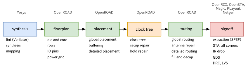
bs_reg in this chapter has 76 steps.
A YAML file configures the run: the name of the top module, the RTL files, the clock, the constraints, the floorplan, and the corners. Everything it does not set comes from the defaults of LibreLane and of the PDK, which libs.tech/librelane/ of SG13CMOS5L holds. The configuration of bs_reg uses the SDC file of Section 6.6 for placement, routing, and signoff, a core with 50 % utilization, and the supply nets VDD and VSS of the AMS chip template. The corners come from the PDK: the typical, slow, and fast corners of Section 5.6 for the nominal supply of 1.2 V, with the typical one as the default corner, which the timing reports between the steps use. LibreLane names each corner after the corner of the wires and the corner of the library, e.g., nom_typ_1p20V_25C for nominal wires and the typical library at 1.2 V and 25 °C:
bs_reg/config.yaml
# SPDX-FileCopyrightText: 2026 Simon Dorrer
# SPDX-License-Identifier: Apache-2.0
# Description: LibreLane configuration of the barrel shifter between
# two registers (bs_reg, 32 bits) of chapter 6. Usage, in this folder:
#   librelane config.yaml --pdk ihp-sg13cmos5l --pdk-root $PDK_ROOT \
#     --manual-pdk --run-tag base
# The run lands in runs/base, its results in runs/base/final.

meta:
  version: 3
  flow: Classic

DESIGN_NAME: bs_reg
VERILOG_FILES:
  - dir::../../../verification/code/barrel_shift/rtl/barrel_shift.sv
  - dir::../../../sequential/code/bs_reg/rtl/bs_reg.sv

# The clock and the constraints of chapter 6
CLOCK_PORT: clk_i
CLOCK_PERIOD: 4.0
PNR_SDC_FILE: dir::../../../sequential/code/bs_reg/syn/bs_reg.sdc
SIGNOFF_SDC_FILE: dir::../../../sequential/code/bs_reg/syn/bs_reg.sdc

# Floorplan: the core takes the cells at the target utilization
FP_SIZING: relative
FP_CORE_UTIL: 50
PL_TARGET_DENSITY_PCT: 60

# The supply nets, named as in the AMS chip template
VDD_NETS: [VDD]
GND_NETS: [VSS]

# The library; its corners come from the PDK: typical, slow, and fast
# at 1.2 V, with the typical one as the default corner
STD_CELL_LIBRARY: sg13cmos5l_stdcell

# Setup violations fail the run in the typical corners only, the
# default of the PDK in image 2026.10. Newer PDKs check all corners.
TIMING_VIOLATION_CORNERS: ["*typ*"]
The run takes about six minutes. LibreLane writes each step into its own numbered folder of the run folder runs/base/, e.g., 06-yosys-synthesis/ or 35-openroad-cts/, with the log of the tool, its reports, the exact commands in COMMANDS, and the state it hands on. The folder final/ collects the results: the layout as GDSII (gds/), as DEF (Design Exchange Format, def/), and as OpenROAD database (odb/), the LEF abstract of the macro for a parent design (Section 5.3, lef/), the netlist without and with supply connections (nl/, pnl/), the extracted parasitics as SPEF (Standard Parasitic Exchange Format, spef/), the delays for a gate-level simulation per corner as SDF (Section 4.10.2, sdf/), a timing model of the macro (lib/), the SPICE netlist extracted from the layout (spice/), and all metrics of the run in metrics.json.
10.2.1 The OpenROAD GUI
The reports give the numbers of a run, and the GUI of OpenROAD shows the layout behind them. LibreLane opens a finished run in it with a flow of one step, OpenInOpenROAD, which needs the desktop of the container (Section 1.13):
librelane config.yaml --pdk ihp-sg13cmos5l --pdk-root $PDK_ROOT \
  --manual-pdk --run-tag base --flow OpenInOpenROAD
The step reads the state that the last step of the run handed on, whose layout database equals the one in final/odb/, and the Liberty files, the SDC file, and the SPEF file of the default corner, with the propagated clock. The GUI therefore shows the timing of the typical corner only, and -c DEFAULT_CORNER=nom_slow_1p08V_125C opens the run in the slow corner instead. The GUI flow writes into the run like any other flow. Each time, it adds a numbered folder for its step, e.g., 77-openroad-opengui/, appends its log to flow.log, saves the state that it opened into final/ again, and replaces resolved.json, the complete configuration of the run, with its own, which no longer shows the settings of the Classic flow. The file config.json in the folder of each step keeps the settings that this step used.
Figure 58 shows the window. The layout fills the middle, with a scale bar at the bottom left. The Display Control on the left switches layers, nets, instances, rows, and heat maps on and off, and a double click on an underlined entry opens its settings. On the right, the Inspector shows the properties of the object under the last click, here the input buffer input1: its cell, its position, its orientation, and its pins. The tabs next to it hold the Hierarchy Browser, the Timing Report, and the Charts, and the menu Windows opens more, such as the Clock Tree Viewer. The Scripting pane at the bottom accepts every command of OpenROAD and OpenSTA, e.g., report_checks of Section 6.7, and shows the files that the step read.
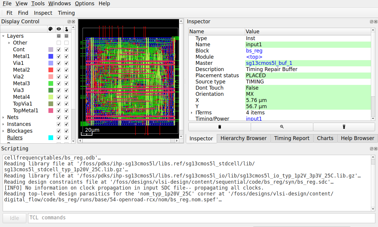
base of bs_reg, as LibreLane opens it: the Display Control on the left, the layout in the middle, the Inspector with the selected input buffer input1 on the right, and the Scripting pane with the files that the step read at the bottom.
10.3 Floorplan
The die is the rectangle of the macro, the core the area inside it where the cells stand. The margins between them hold the pins and, in a chip, a ring of supply wires. With FP_SIZING: relative, LibreLane derives the core from the area of the synthesized cells: FP_CORE_UTIL: 50 makes the core twice as large as the cells, and the core is square unless an aspect ratio is set. The free half is not wasted. Placement adds buffers, clock tree synthesis adds a tree, timing repair enlarges cells, and the router needs free tracks above the cells. The other way is FP_SIZING: absolute with a fixed DIE_AREA, as in the counter of the AMS chip template.
The core is divided into rows of the height of a cell, 3.78 µm in SG13CMOS5L, made of sites of 0.48 µm width (Section 5.3). Every cell is a whole number of sites wide. Every second row is flipped, so that two neighboring rows share their supply rail. Many libraries, e.g., ETH LV (Section 5.3.4), need tap cells in every row, which tie the wells and the substrate to the supplies. The cells of IHP LV contain these ties themselves (Section 5.3.2), so the PDK sets FP_TAPCELL_DIST to 0, and the flow inserts none.
The power distribution network (PDN) brings VDD and VSS to every row (Figure 59). Metal1 rails run along the rows, where the cells connect to them. Vertical straps on Metal4, 1 µm wide every 50 µm, connect to the rails through stacks of vias, and horizontal straps on TopMetal1, 2 µm wide every 50 µm, connect to the Metal4 straps. The straps of both layers form the supply pins of the macro, to which the parent connects its own grid. The pins of the signals sit on the edges of the die, on Metal3 on the left and right and on Metal2 at the top and bottom, the layers whose preferred direction leads into the core. The IO placer orders them to keep the wires short, or follows a pin order file.
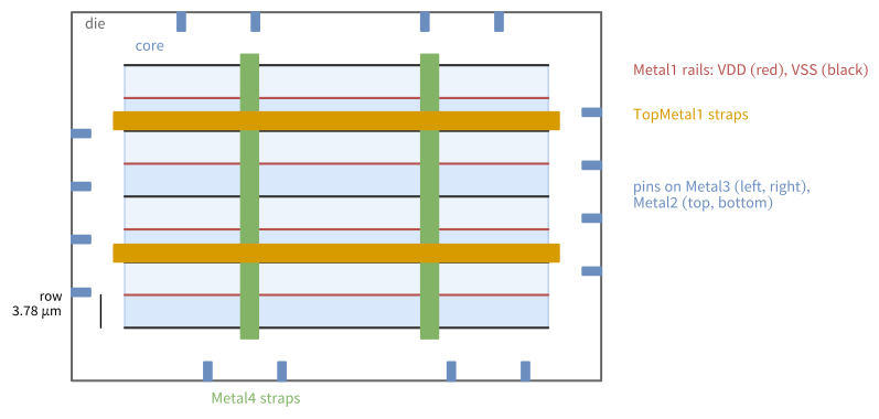
TipExercise: Plan the Floorplan
All commands start in the folder content/digital_flow/code/bs_reg. Start the run first, it takes about six minutes:
librelane config.yaml --pdk ihp-sg13cmos5l --pdk-root $PDK_ROOT \
  --manual-pdk --run-tag base
Sketch the floorplan of
bs_regwith the core, the rows, the straps, and the pins, and add the numbers: the synthesis reportruns/base/06-yosys-synthesis/reports/stat.rptgives the area of the synthesized cells. Compute the core for 50 % utilization, its edge for a square core, and the number of rows and sites that fit.Compare with the layout:
runs/base/final/def/bs_reg.defholds the die (DIEAREA) and oneROWstatement per row, in database units of 1 nm. How large are the die and the core, and how wide are the margins? Which utilization and cell area doesruns/base/final/metrics.jsonreport for the finished layout (design__instance__utilization,design__instance__area__stdcell), and how much area did the steps after the synthesis add?Open the run in the GUI (Section 10.2.1), hide the signal and clock nets under
Netsin the Display Control, and compare the straps on Metal4 and TopMetal1 with your sketch. A click on a strap shows its net in the Inspector, and the status bar at the bottom shows the coordinates under the pointer. Where do the straps ofVDDandVSSlie (the sectionSPECIALNETSof the DEF file gives the exact positions), and why doesVSShave one Metal4 strap less?Run the flow again with a denser core and a higher density limit for the placement (
PL_TARGET_DENSITY_PCT, Section 10.4):librelane config.yaml --pdk ihp-sg13cmos5l --pdk-root $PDK_ROOT \ --manual-pdk --run-tag util75 \ -c FP_CORE_UTIL=75 -c PL_TARGET_DENSITY_PCT=85How do the utilization, the wire length (
route__wirelength), the number of iterations of the detailed router (Section 10.6,route__drc_errors__iter:N), and the worst setup slack in the typical corner change? Is a smaller core worth it here?
Before continuing, please finish the previous exercise. Once you are done, compare with the solution below.
TipSolution: Plan the Floorplan
- The synthesized cells take 13,008.1 µm², so the core needs 26,016 µm², an edge of 161.3 µm. That fits 42 rows of 3.78 µm (158.76 µm) and 336 sites of 0.48 µm (161.28 µm). Metal1 rails run along the rows. Over the 161 µm of the core, the Metal4 straps every 50 µm make 4 for
VDDand 3 forVSS, and TopMetal1 has 3 pairs. The pins sit on all four edges. - The rows fill 161.28 µm × 158.76 µm, 25,604.8 µm², with 42 rows of 336 sites. The die is 172.82 µm × 191.54 µm: the computed edge of 161.30 µm plus margins of 12 sites (5.76 µm) left and right and of 4 rows (15.12 µm) at the bottom and top. Of the computed square, 0.02 µm at the right and 2.54 µm at the top do not fill a whole site or row and stay empty. The finished layout reports 58.7 % utilization, 15,023.2 µm² of cells, because placement, clock tree synthesis, and timing repair added 2015 µm² of buffers and larger cells.
- Every
VDDstrap has aVSSstrap next to it. On Metal4, the 1 µm wide straps of the first pair have their centers at x = 15.76 µm and 18.76 µm, and a pair follows every 50 µm. On TopMetal1, the 2 µm wide straps of the first pair lie at y = 25.12 µm and 31.12 µm, again every 50 µm. The fourth Metal4 pair would place itsVSSstrap at x = 168.76 µm, beyond the right edge of the core at 167.04 µm, so only itsVDDstrap at 165.76 µm remains. - With 75 %, the core shrinks to 16,903 µm², and the finished layout fills 89.2 % of it. The detailed router starts with 1139 instead of 683 violations and needs 6 instead of 4 iterations, the wire length grows from 40,693 to 45,974 µm, and the worst setup slack in the typical corner drops from 1.075 to 0.997 ns. The core is 34 % smaller, but harder to route and slower. For a macro that the parent places in a fixed slot, the margin is worth more.
10.4 Placement
Global placement spreads the cells over the core so that the total wire length is short and no region is denser than PL_TARGET_DENSITY_PCT. OpenROAD treats the cells like charges that repel each other, while the nets pull connected cells together, and the result still allows overlaps. After it, OpenROAD can estimate the wires for STA: it approximates each net by a tree through its pins and multiplies the length by a resistance and a capacitance per micron. LibreLane takes both from the technology LEF, averaged over the routing layers Metal2 to TopMetal1: 0.389 Ω/µm and 0.097 fF/µm, against 0.515 Ω/µm and 0.093 fF/µm for Metal2 alone.
Then the repair of the design fixes every net that breaks a limit of the library or the constraints: the maximum slew, the maximum capacitance, and the maximum fanout. The SDC of bs_reg sets no fanout limit, so the default of the Liberty file applies, 8 loads (default_max_fanout). A design without an SDC file of its own gets the SDC of LibreLane, which sets the 10 loads of the PDK (MAX_FANOUT_CONSTRAINT). For bs_reg, OpenROAD first puts a buf_1 behind each of the 40 inputs and in front of each of the 32 outputs, which separates the inside of the macro from its surroundings. It then finds 5 nets with too slow a slew and 30 nets with more than 8 loads, and inserts 142 more buffers into them. Synthesis did not do this: LibreLane’s default synthesis strategy, AREA 0, lets ABC insert buffers only when SYNTH_ABC_BUFFERING is set, which is off by default, so its netlist has no buffers at all (Section 5.7). Detailed placement finally moves every cell onto a site of a row, without overlaps.
10.5 Clock Tree Synthesis
Until now, the timing analyses of our designs assumed an ideal clock that reaches every flip-flop at the same moment (Section 6.6). In reality, one clock pin cannot drive dozens of flip-flops spread over the core. Clock tree synthesis (CTS) builds a tree of buffers from the clock pin to every flip-flop, so that the clock edge reaches all of them after about the same delay, the latency, with a small difference, the skew. TritonCTS, the CTS of OpenROAD, builds an H-tree: it divides the region of the flip-flops recursively into halves, connects the halves with branches of equal length, and places buffers along the tree that drive the branches and the flip-flops. It chooses from the clock buffers that the PDK lists, buf_8 down to buf_1, with buf_8 at the root. From now on, STA uses the propagated clock, i.e., the real arrival time of the clock at each flip-flop.
Skew moves time from one check to the other (Section 6.10): a capturing flip-flop whose clock arrives late gains setup time and loses hold time. After CTS, OpenROAD therefore repairs the timing with the real clock: it enlarges cells and adds buffers on paths that violate setup, and it inserts delay cells, dlygate4sd1_1 to dlygate4sd3_1, into paths that violate hold, up to the margins PL_RESIZER_SETUP_SLACK_MARGIN and PL_RESIZER_HOLD_SLACK_MARGIN (0.05 and 0.1 ns by default). The candidates for hold violations are short paths, in which one flip-flop drives the next directly, as in the scan chains of Section 9.
A clock gate (Section 7.7) sits inside the clock tree, and the flip-flops behind it see its delay on top of the tree. TritonCTS balances this extra delay. The design cg_mix has two 16-bit registers on one clock, one of them behind an lgcp_1. CTS builds one tree behind the clock gate and one for the ungated register, reports that it balances the latency of the clock, and inserts three buf_8 as delay buffers in front of the tree of the ungated register. In the typical corner, the rising clock edge then reaches all 32 flip-flops between 0.440 and 0.442 ns after the clock pin.
A divided clock (Section 3.4.2) gets no such help. In div_mix, a flip-flop divides clk_i by two, and a 16-bit register on the divided clock takes over the value of a register on clk_i. Its SDC file defines the divided clock with create_generated_clock (Section 6.8). CTS finds two clock nets, clk_i and the output div_q of the divider, and builds a tree for each without balancing them against each other. The flip-flops behind the divider therefore see the clock later, by the clock-to-output delay of the divider and the delay of the second tree, and after CTS all 16 paths from clk_i into the divided clock violate hold, by up to 0.25 ns in the typical corner. The timing repair fixes them with 32 delay cells, two in front of each flip-flop. A clock enable on clk_i needs neither the second tree nor the delay cells.
The Clock Tree Viewer of the GUI (menu Windows) draws the tree of each clock in a tab of its own, named after the clock of the SDC file, after a click on Update (Figure 60 and Figure 61). The source of the clock sits at the top, and each buffer and each flip-flop sits at the latest time when the rising clock edge reaches it, in the corner chosen at the top left, so a balanced tree ends in one flat row of flip-flops. In cg_mix, the gated branch passes two buf_8, the clock gate (drawn as a circle), and one more buf_8 before its four leaf buffers, and the ungated branch passes the three delay buffers and two more buf_8. Both end in the same row, at 0.44 ns. In div_mix, the tab clk shows the 17 flip-flops on clk_i, the divider included, which see the edge after about 0.14 ns. The tab clk_div starts at the output of the divider, after about 0.3 ns, and its 16 flip-flops see the edge only after about 0.49 ns. This difference causes the hold violations, which the repair fixes with delay cells.
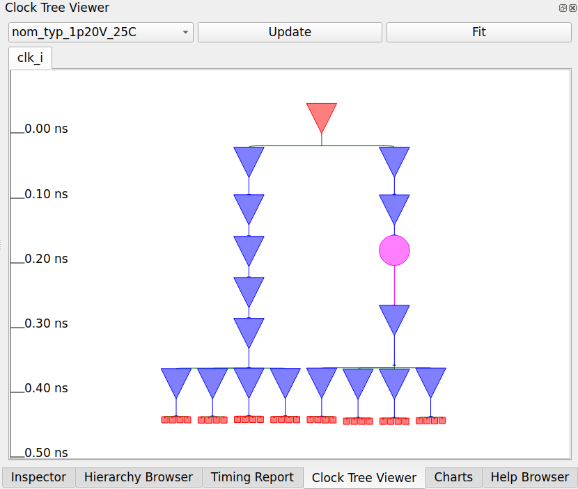
cg_mix in the typical corner, with the time running downward: the clock source (red triangle), the buffers (blue triangles), the clock gate (pink circle) in one branch, three delay buffers in the other, and the flip-flops (red squares).
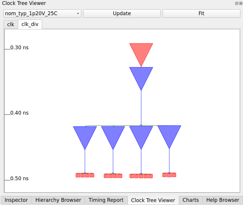
clk_div of div_mix: the tree of the divided clock starts at the output of the divider.
TipExercise: Follow the Clock and the Reset
All commands start in the folder content/digital_flow/code/bs_reg and use the run base of the previous exercise.
Sketch the clock tree of
bs_regfrom the log of CTS,runs/base/35-openroad-cts/openroad-cts.log: how many flip-flops does it drive, how many buffers did it create, how many buffers are in each clock path, and how many flip-flops does each last buffer drive? What are the dummy loads that CTS reports?Open the run in the GUI and its Clock Tree Viewer, and compare the tree with your sketch. Between which times does the clock edge reach the flip-flops? Compare this spread with the latencies in
clock.rptin the folder of the typical corner,runs/base/55-openroad-stapostpnr/nom_typ_1p20V_25C/, and with the worst setup skew of the corner inruns/base/final/metrics.json(clock__skew__worst_setup__corner:...). The fileskew.max.rptin the same folder shows how STA computes its skew.Which output drives the only fanout violation of the run (
checks.rptin the same folder), and why did the repair of the design not fix it?The reset input
rst_nidrives theRESET_Bpins of all flip-flops. Follow it in the final netlistruns/base/final/nl/bs_reg.nl.v: how many buffers lie betweenrst_niand a flip-flop at most, and how manyRESET_Bpins does one buffer drive at most? How large is the worst recovery slack in the typical and the slow corner? The path that starts atrst_niin the filemax.rptof each corner shows it.No path needed a hold repair. Ask for a larger hold margin and run again:
librelane config.yaml --pdk ihp-sg13cmos5l --pdk-root $PDK_ROOT \
  --manual-pdk --run-tag hold05 \
  -c PL_RESIZER_HOLD_SLACK_MARGIN=0.5
Which of the delay cells did the flow choose, how many did it insert, and how much area do they cost? Is the margin reached?
Before continuing, please finish the previous exercise. Once you are done, compare with the solution below.
TipSolution: Follow the Clock and the Reset
- The clock net
clk_ihas 71 sinks. CTS builds an H-tree with 17buf_8: one at the root, which drives 16 leaf buffers, and each leaf drives 4 or 5 flip-flops (9 × 4 + 7 × 5 = 71). Every clock path has exactly 2 buffers. The 9 leaves with only 4 flip-flops get a dummy load, aninv_1whose output stays open, so that all 16 leaves carry about the same load and the same delay. Together they make the 80 sinks that the log reports. - The viewer shows the tree of the sketch (Figure 62): the root, 16 leaves, and the 71 flip-flops in one row, reached between 0.237 and 0.250 ns, a spread of only 0.013 ns.
clock.rptgives 0.225 to 0.250 ns, because STA computes an early and a late arrival at each flip-flop. The early analysis takes the smaller value of each pin capacitance, which the library gives as a range (rise_capacitance_range), and the report combines the early arrival at_1508_with the late one at_1482_. The viewer draws the late arrivals only. The worst setup skew inmetrics.jsonis 0.118 ns in the typical corner, 0.124 ns in the slow and 0.116 ns in the fast one.skew.max.rptshows how STA gets there: it takes the late clock at a launching flip-flop (0.250 ns at_1482_) minus the early clock at a capturing one (0.225 ns at_1508_), adds the clock uncertainty of 0.1 ns from the SDC (Section 6.4), and subtracts 0.007 ns of clock reconvergence pessimism, the early and late difference on the part that both clock paths share (Section 6.7). The metric is a margin for the setup check, not the spread of the tree. - The fanout violation belongs to the root buffer
clkbuf_0_clk_i, which drives 16 leaves against a limit of 8. The repair of the design ran before CTS and skips clock nets anyway, and CTS groups the sinks by the load its buffers can drive, not by the fanout limit. - The repair of the design turned the reset net into a tree of 13
buf_1, the input buffer included, and theRESET_Bpins hang on 12 of its nets, with 2 to 8 pins each. At most five buffers lie betweenrst_niand a flip-flop. In Section 6.7, onebuf_2drove all 71 pins with a slew of 0.87 ns. The tree splits this load, at the price of more delay, which the recovery check easily allows: its worst slack is 1.912 ns in the typical and 1.356 ns in the slow corner. - The flow inserts 131
dlygate4sd3_1, the delay cell with the largest delay, and the area of the cells grows by 14 %, from 15,023.2 to 17,162.4 µm². The resizer still warns that it cannot repair all hold checks within the margin: it reaches only 0.22 ns on its estimates, and at signoff the fast corner has 0.268 ns, far below the 0.5 ns asked for. Hold margin costs area, so the default asks for 0.1 ns only.
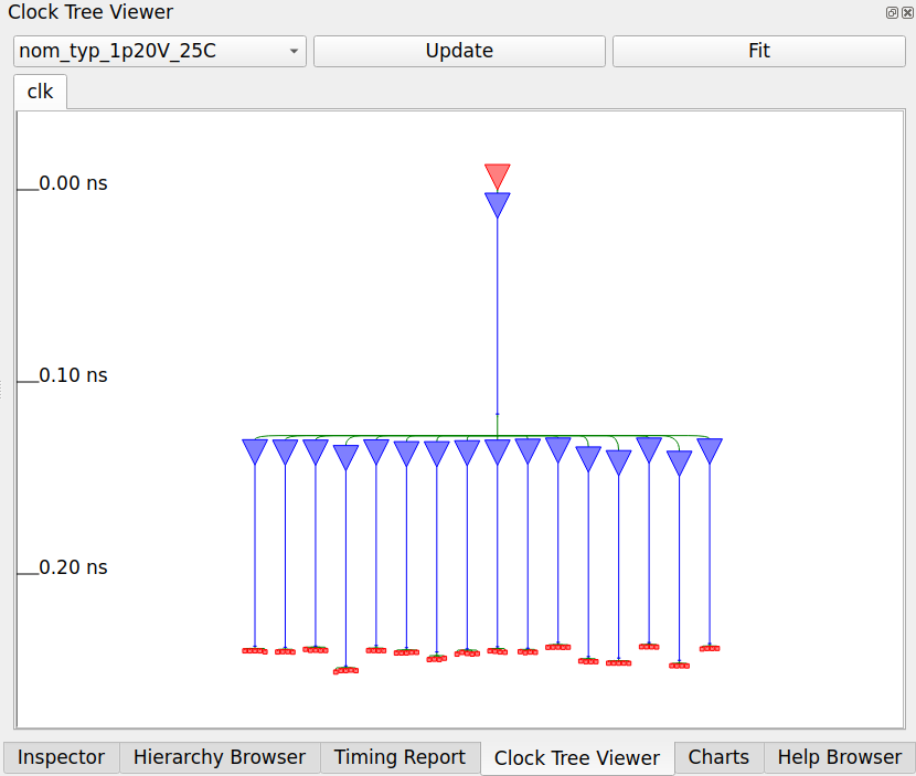
bs_reg in the Clock Tree Viewer, typical corner: the clock pin, the root buf_8, 16 leaf buffers, and the 71 flip-flops between 0.237 and 0.250 ns.
10.6 Routing
Global routing divides the die into a grid of tiles, assigns each net a path through the tiles and a layer, and counts the demand of each tile against its tracks. A tile with more demand than tracks is congested, and the router detours nets around it. For bs_reg, the global router uses 44 % of the tracks of Metal2 and 39 % of Metal3, 28 % of all tracks, without overflow, i.e., no tile is congested. STA can now use the global routes instead of the estimates of the placement. LibreLane can also repair the timing once more on them, but this step (RUN_POST_GRT_RESIZER_TIMING) is off by default. Global routing also checks the antenna rule: while a wire is being manufactured, it collects charge, and a long wire that ends at a gate can damage the gate oxide before the upper metal connects it to a diffusion that drains the charge. The fix is a jumper to a higher layer or a diode cell, antennanp in SG13CMOS5L, next to the gate. bs_reg has no violation and needs no diode.
Detailed routing with TritonRoute draws every wire on the tracks of its layer, with the widths, spacings, and vias that the design rules demand. It starts from a first solution with violations and repairs them in iterations: for bs_reg, 683 violations after the first iteration, then 355 and 296, and none after the fourth. The routed wires are 40,693 µm long, and the longest net 436 µm.
After routing, fill insertion closes the gaps in the rows with filler cells, which continue the wells and the rails, and with decoupling capacitors (Section 5.3): 634 decap_8 and 151 decap_4, which hold charge between VDD and VSS where cells switch, and 255 fill_2 and 280 fill_1 in the gaps that are too small for them. Figure 63 shows the finished layout.
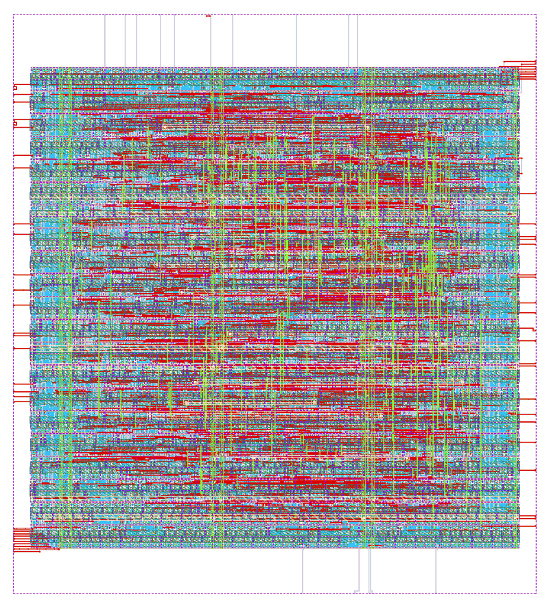
bs_reg, 172.82 µm × 191.54 µm, rendered by LibreLane. The rows of cells fill the core, the signal wires run vertically on Metal2 and Metal4 and horizontally on Metal3 and TopMetal1, and the pins sit on the edges of the die.
The GUI shows the global routing as a heat map, Routing Congestion under Heat Maps in the Display Control. It reads the grid of tiles that the global router stores in the layout database, 7.2 µm wide for bs_reg, and colors each tile by the share of its routing capacity in use: for all layers, the larger share of the two directions, horizontal (Metal3 and TopMetal1) and vertical (Metal2 and Metal4), or, after a double click on the entry, the share of one layer. To see the map that the global router left, open the state that its step handed on, with --with-initial-state, under a run tag of its own:
librelane config.yaml --pdk ihp-sg13cmos5l --pdk-root $PDK_ROOT \
  --manual-pdk --run-tag base_grt --flow OpenInOpenROAD \
  --with-initial-state \
  runs/base/39-openroad-globalrouting/state_out.json
The own run tag matters. The GUI step hands on the state that it opened and saves it into final/ of its run. In the run base itself, the layout and the metrics in final/ would turn into those of the global routing, and every later GUI session would open the global routing again. base_grt gets only the folder of the GUI step and its own final/. gui::dump_heatmap Routing heat.csv in the Scripting pane writes the value of every tile into a file.
Figure 64 shows the map of base with the signal and clock nets hidden. The middle of the core is the fullest, 82 % on average in the middle half of the core in x and in y, against 38 % in the margins around the core, and 10 tiles reach 100 %, 8 of them in the middle. A full tile uses all its tracks, but it is not congested, because no tile overflows. The other heat maps work the same way: the placement density, RUDY (Rectangular Uniform wire Density, a quick estimate of the routing demand from the placement alone), the power density, the pin density, and the IR drop of Section 10.7.
bs_reg after global routing in the OpenROAD GUI, with the signal and clock nets hidden and the legend at the top right. The middle of the core is the fullest.
TipExercise: Find the Congestion
All commands start in the folder content/digital_flow/code/bs_reg and use the runs base and util75 of the first exercise.
Sketch the core of
util75next to the core ofbasefrom the first exercise, at the same scale, and shade where you expect the routing to be fullest.Open
util75at the state after global routing and show its routing congestion map:librelane config.yaml --pdk ihp-sg13cmos5l --pdk-root $PDK_ROOT \ --manual-pdk --run-tag util75_grt --flow OpenInOpenROAD \ --with-initial-state \ runs/util75/39-openroad-globalrouting/state_out.jsonWhere are the full tiles now, and how many tiles reach 90 % and 100 %, compared with
base? Count them in the file ofgui::dump_heatmap. Compare the usage per layer in the log of the global routing of both runs, the table afterGRT-0096inruns/<run>/39-openroad-globalrouting/openroad-globalrouting.log.Choose Metal4 alone in the settings of the map. Why does the map of
util75show bright columns, and why does it read 30 % or more even between them, although the log ofutil75gives Metal4 only 13 % of usage?Open the final state of
util75with--run-tag util75and without--with-initial-state, and show the map again. What do you see, and why does this chapter open the state of the global routing for this map?
Before continuing, please finish the previous exercise. Once you are done, compare with the solution below.
TipSolution: Find the Congestion
- The denser core holds the same cells and nets on a third less area, so expect more demand everywhere, and most of it in the middle, as in
base. - After global routing, the map of
util75is full almost everywhere in the core (Figure 65): 152 of its 418 tiles reach 90 % or more and 33 reach 100 %, against 60 of 624 and 10 inbase, and the margins around the core reach 57 % on average instead of 38 %. The log agrees. The global router uses 45.65 % of all tracks instead of 28.20 %, 58.89 % of Metal2 and 64.18 % of Metal3 instead of 43.96 % and 38.85 %. No tile overflows, but full tiles leave the router no room for detours, so the detailed router starts with 1139 instead of 683 violations (first exercise). - The bright columns lie on the Metal4 straps of the power grid, at x = 16, 66, and 116 µm, where the map reads 57 to 68 % instead of 31 to 48 % between them. The map counts the tracks under a strap as used. It also counts the 30 % of the tracks of every layer that the global router keeps free for the detailed router (
GRT_ADJUSTMENTof 0.3 inconfig.jsonof the step), so even a layer with few wires reads 30 % or more. The log counts only the tracks that are left, and of those the routes use 13 % on Metal4. - The final database of
util75holds a different map (Figure 66): at most 57 %, 38 % on average, cooler thanbaseafter global routing. Inutil75, the antenna repair after global routing found 6 violations, inserted 6 diodes, and routed the affected nets again (42-openroad-repairantennas/), and the global router then stored a new grid, in which most tiles hold little more than the reserve and the straps.basehas no antenna violation, so it keeps the map of the global routing, which makes the difference easy to miss. The map of a final state need not show the global routing, so open the state of the global routing for it, and compare it with the log of the global router.
util75 after global routing in the OpenROAD GUI, with the signal and clock nets hidden.
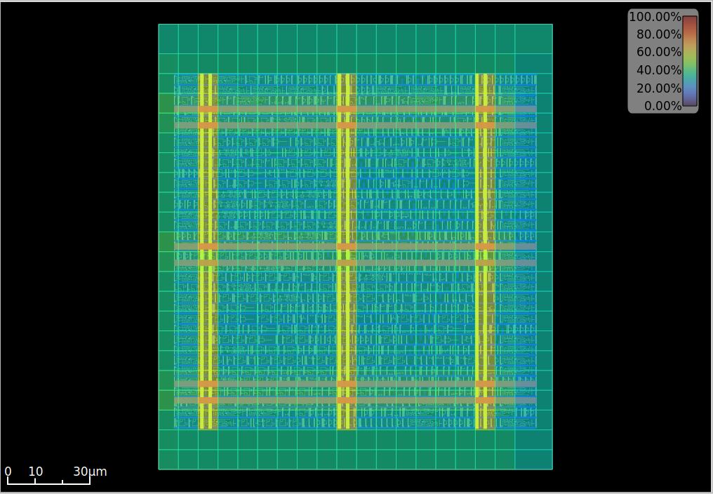
util75 in the final database, with the same settings.
10.7 Signoff
Only now are the wires known. Parasitic extraction with OpenRCX computes the resistance of every wire and its capacitance to ground and to its neighbors from the routed layout and the rules of the PDK, and writes them as SPEF. STA reads the SPEF instead of the estimates, and it writes SDF files with the delays of every cell and every wire, which a gate-level simulation can back-annotate (Section 10.8). The signoff STA checks setup and hold in every corner, the slow corner for setup and the fast one for hold in particular, and LibreLane collects the results in 55-openroad-stapostpnr/summary.rpt.
Figure 67 follows the worst setup slack through the run. The synthesized netlist misses the 4 ns clock, because ABC left the high-fanout nets unbuffered. After the repair of the design and CTS, the slack is positive, and the timing repair adds to it. Then the slack shrinks again, from 1.45 ns after the timing repair to 1.08 ns: the global routes cost 0.11 ns, and the extracted wires another 0.26 ns. The estimates before routing are optimistic: real wires take detours and change layers through vias, and the extraction counts the capacitance between neighboring wires, which the estimate per micron does not.
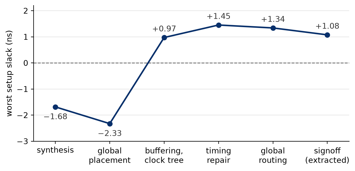
bs_reg at 250 MHz in the typical corner after each stage of the LibreLane run, from its STA steps. The synthesized netlist misses the clock because its high-fanout nets are not buffered. Placement adds the estimated wires. Buffering, clock tree synthesis with the propagated clock, and the timing repair raise the slack. The global routes and, after routing, the extracted wires take some of it back.
The Timing Report of the GUI lists the worst paths of the default corner for setup and hold. Update fills the list, and a click on a path draws it into the layout: the clock path of the launching flip-flop, the data path, and the clock path of the capturing flip-flop, each in its own color, while the table below lists the path pin by pin, as max.rpt does. The Charts show how many endpoints reach which slack (Endpoint Slack). Both cover the default corner only (Section 10.2.1).
Besides timing, the signoff checks the layout itself:
- IR drop. OpenROAD computes the voltage drop in the power grid for the estimated currents of the cells. The worst drop on
VDDinbs_regis 1.33 mV, 0.11 % of the 1.2 V supply, andVSSrises by at most 1.99 mV. - DRC. Magic and KLayout check the GDSII against the design rules of the PDK, with 0 violations each for
bs_reg. KLayout also compares the GDSII files that Magic and KLayout stream out (an XOR, 0 differences). - LVS. Magic extracts a netlist from the layout, and Netgen compares it with the netlist with supply connections (
pnl/): “Circuits match uniquely”. In the flow, the cells are abstracts, boxes with their pins and nothing inside, so the comparison covers the connections between the cells and not the transistors inside them. The AMS chip template can also run a full LVS of the GDSII with KLayout (make klayout-lvs). - Antenna. A second antenna check on the routed layout, with 0 violations.
In the GUI, analyze_power_grid -net VDD in the Scripting pane repeats the IR drop analysis of the flow, and the heat map IR Drop then shows where the drop arises (Figure 68). On VDD, it is largest in the top rows of the core, at about x = 50 µm and y = 155 µm, halfway between two Metal4 straps. The configuration of bs_reg names no voltage sources (VSRC_LOC_FILES), so OpenROAD holds the pins of the net at the supply voltage, here all straps on Metal4 and TopMetal1 (Section 10.3), and the drop arises only in the via stacks and the Metal1 rails between them. warning.log warns that this may make the result inaccurate, and adds that only a top-level chip for manufacture needs to care.
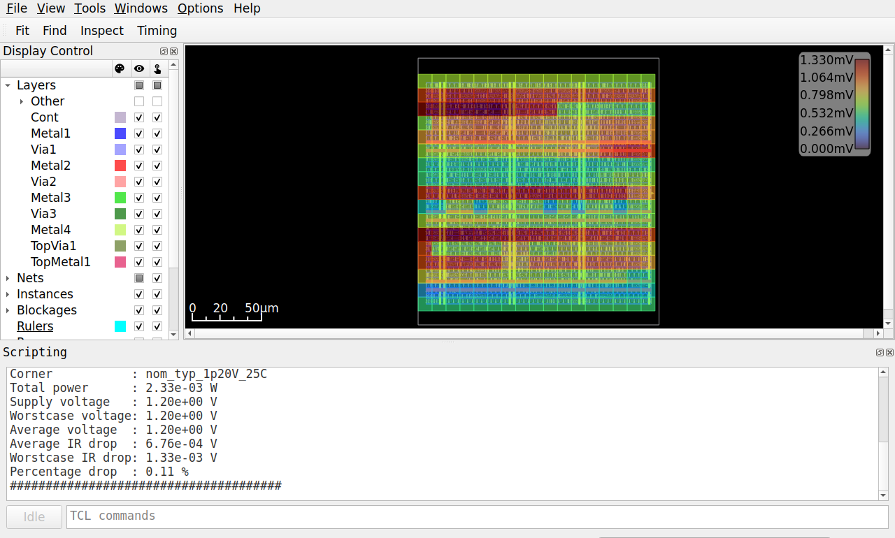
VDD in bs_reg in the OpenROAD GUI after analyze_power_grid -net VDD, with the signal and clock nets hidden: the map with its legend in mV, and the report of the analysis in the Scripting pane.
One more check proves that the netlist still does what the RTL describes. The layout flow changed it: buffers, a clock tree, resized cells, and delay cells. LibreLane’s own equivalence step prepares the cell models only for sky130, so we run EQY ourselves on the final netlist, with the setup of Section 5.8. Flattening the RTL keeps the net names of the submodule u_shift as second names of the nets of bs_reg, which would confuse the matching, so both sides hide the hierarchical names:
bs_reg/lec.eqy
# SPDX-FileCopyrightText: 2026 Simon Dorrer
# SPDX-License-Identifier: Apache-2.0
# Description: Equivalence check of bs_reg: its RTL (gold) against the
# final netlist of the LibreLane run in runs/base (gate). Run in this
# folder with stdcell.lib linked to the typical library of SG13CMOS5L:
# eqy -d lec_eqy lec.eqy

[gold]
plugin -i slang
read_slang --top bs_reg \
  ../../../verification/code/barrel_shift/rtl/barrel_shift.sv \
  ../../../sequential/code/bs_reg/rtl/bs_reg.sv
hierarchy -check -top bs_reg
proc
flatten -noscopeinfo
# Flattening keeps the net names of the submodule as second names
rename -hide w:*.*

[gate]
# The cell functions come from the Liberty file
read_liberty -ignore_miss_func stdcell.lib
read_verilog runs/base/final/nl/bs_reg.nl.v
hierarchy -check -top bs_reg
flatten -noscopeinfo
# Fails if a cell had no model and stayed a black box
select -assert-none t:sg13cmos5l_*
rename -hide w:*.*

[strategy sby]
use sby
engine abc pdr
TipExercise: Close the Timing
All commands start in the folder content/digital_flow/code/bs_reg and use the run base of the first exercise.
Sketch the worst path of the failing corner. Open
runs/base/55-openroad-stapostpnr/summary.rpt: which corner fails, by how much, and at how many endpoints? Then draw the worst path of that corner from the filemax.rptin the folder of the corner: where does it start, through which cells does it run, and where does it end?Open the run in the GUI in the failing corner (
-c DEFAULT_CORNER=<corner>, Section 10.2.1) and draw the worst setup path of the Timing Report into the layout.Findin the toolbar selects an instance by its name, and the Inspector shows its position. Where on the die do the first and the last flip-flop of the path sit, and why does the path cross so much of the core? ChooseEndpoint Slackin the Charts: does the histogram agree withsummary.rpt, and how many endpoints fail by more than 0.5 ns?The timing repair after CTS worked on all corners. Read its log,
runs/base/37-openroad-resizertimingpostcts/openroad-resizertimingpostcts.log: from which worst slack did it start, and which did it reach? How much slack did the slow corner lose between the repair and signoff, compared with the typical corner in Figure 67?Try a delay-oriented synthesis first,
-c SYNTH_STRATEGY="DELAY 4"with--run-tag delay4. What happens to the slack in the slow corner and to the area of the cells (design__instance__area__stdcell)?Ask the repair for a setup margin of 0.6 ns,
-c PL_RESIZER_SETUP_SLACK_MARGIN=0.6with--run-tag margin. Why this value? Do all corners pass now, and at which cost in area?The resizer changed the netlist. Prove that the final netlist of
runs/basestill implements the RTL:ln -sf $LIB stdcell.lib eqy -f -d lec_eqy lec.eqyWhat does EQY report? Then replace the first
sg13cmos5l_a21oi_1in the file bysg13cmos5l_o21ai_1in a copy of the netlist, pointread_verilogin a copy oflec.eqyto it, and check again.
Before continuing, please finish the previous exercise. Once you are done, compare with the solution below.
TipSolution: Close the Timing
- The slow corner fails with a worst setup slack of -0.586 ns at 31 endpoints, with a total of -6.98 ns, while the typical corner has 1.075 ns and the fast corner 2.072 ns. Hold passes everywhere, with 0.204 ns in the fast corner. The worst path starts at
_1537_, the flip-flop ofshamt_q[1], and ends at the input of a flip-flop ofout_q. Of the 3.59 ns from the output of the first flip-flop to the input of the second, 1.83 ns go into six buffers of the repair of the design: two behind the flip-flop, whose output drove 36 loads before the repair, and a chain of four behind an XNOR gate, whose output drove 53. The rest goes into the XNOR gate, two multiplexers, and four other gates. - The GUI draws the path across the core (Figure 69). It starts at
_1537_in the top left corner, at x = 10.1 µm and y = 162.5 µm, next to the input pinshamt_i[1]that feeds it, and ends at_1516_near the right edge, at x = 153.6 µm and y = 117.2 µm, next to the output pindata_o[12]that it drives. Both flip-flops sit next to their pins, on opposite sides of the die, so the logic between them has to cross the core. The histogram agrees withsummary.rpt: 31 endpoints below 0 ns, 2 of them below -0.5 ns. - The repair started at -0.725 ns, the worst slack over all corners, i.e., in the slow corner, resized 8 cells, removed one buffer, and reached +0.031 ns on its estimates, below its margin of 0.05 ns, so it reported that it could not repair all violations. After routing, the slow corner ends at -0.586 ns, so it lost 0.62 ns on the way to signoff, against 0.38 ns in the typical corner. The estimates before routing are optimistic, and the slow corner suffers most, because its weaker cells turn the same extra capacitance into more delay.
- With
DELAY 4, the slow corner improves only to -0.542 ns, while the area of the cells grows by 12 % to 16,852.1 µm². The synthesis was not the problem: the repair reached 0.088 ns on its estimates, above its margin, and the wires again took 0.63 ns. - The margin covers the loss of about 0.6 ns that the slow corner showed in the third step. With it, all corners pass: 0.048 ns in the slow corner, 1.512 ns in the typical corner. The cells take 15,170.2 µm², only 1 % more than in
base. The right knob depends on the mechanism: here the estimate before routing was the problem, not the logic. - EQY proves the designs equivalent in 32 partitions, one per output bit, in less than half a minute. With the replaced cell, it fails the partitions of two output bits,
data_o[1]anddata_o[17]. The equivalence check belongs after every step that changes the netlist, and the layout flow changes it a lot.
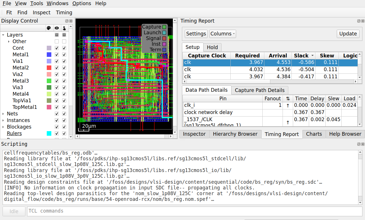
10.7.1 The Reports of a Run
The run base ends with Flow complete., and still its slow corner fails. Besides a step that ends with an error, only a failing checker makes a run fail (Section 10.2), and each checker of the timing counts only the corners in its own variable. The configuration sets TIMING_VIOLATION_CORNERS to the typical corners (*typ*), the default of the PDK in the image 2026.10, so the checker of the setup violations only warns about the slow corner in flow.log and warning.log. Newer versions of the PDK set all corners (*), and without the line in the configuration, the same run then ends with an error. HOLD_VIOLATION_CORNERS covers all corners (*), so a hold violation in any corner fails the run, and the checkers of the maximum slew and capacitance count no corner at all. The report manufacturability.rpt at the end of the run says Passed for antenna, LVS, and DRC, and nothing about the timing. A finished flow is therefore not necessarily a clean design. After every run, read the reports of Table 40, and final/metrics.json, which collects most of their numbers.
base and the questions they answer. <corner> stands for the folder of a corner, e.g., nom_slow_1p08V_125C/.
| Question | Folder in runs/base/ |
Report |
|---|---|---|
| Which steps warned or failed? | the run folder | warning.log, error.log |
| Which settings did a step use? | the folder of the step | config.json |
| How large is the synthesized netlist? | 06-yosys-synthesis/reports/ |
stat.rpt |
| Is the timing met in every corner? | 55-openroad-stapostpnr/ |
summary.rpt |
| Which paths fail, and by how much? | 55-openroad-stapostpnr/<corner>/ |
max.rpt, min.rpt, violator_list.rpt |
| Which slew, capacitance, and fanout limits fail? | the same | checks.rpt |
| How large are the latency and the skew? | the same | clock.rpt, skew.max.rpt |
| How much power does the block take? | the same | power.rpt |
| How large is the IR drop? | 56-openroad-irdropreport/ |
irdrop.rpt |
| Are there antenna violations? | 46-openroad-checkantennas-1/reports/ |
antenna_summary.rpt |
| Does the layout pass DRC? | 64-magic-drc/reports/, 65-klayout-drc/reports/ |
drc.magic.rpt, drc.klayout.json |
| Does the layout match the netlist? | 70-netgen-lvs/reports/ |
lvs.netgen.rpt |
| Do antenna, LVS, and DRC pass? | 76-misc-reportmanufacturability/ |
manufacturability.rpt |
TipExercise: Read the Reports
All commands start in the folder content/digital_flow/code/bs_reg and use the run base of the first exercise.
- Draw the power grid of
bs_regfrom the first exercise again, with the straps ofVDDandVSSon Metal4 and TopMetal1, and mark where you expectVSSto rise most, compared with the drop ofVDDin Figure 68. - Open the run in the GUI, analyze the ground net with
analyze_power_grid -net VSS, and show its map: a double click onIR Dropin the Display Control opens the settings, where you choose the net. Where doesVSSrise most, and why there? Compare the report of the analysis withirdrop.rpt. - Count the lines of
warning.logby their text, withsort runs/base/warning.log | uniq -c. Which warnings concern the run, and which only the tools? - Which group in
power.rptof the typical corner takes the most power, and which share goes into the clock tree?
Before continuing, please finish the previous exercise. Once you are done, compare with the solution below.
TipSolution: Read the Reports
VSShas its straps next to those ofVDDand should behave the same, with one exception: the fourth Metal4 pair on the right has noVSSstrap (first exercise).VSSrises most at the right edge of the core, by 1.99 mV at about x = 160 µm and y = 65 µm (Figure 70), asirdrop.rptreports (Worstcase voltage: 1.99e-03 V). There, the nearest Metal4 strap ofVSS, at x = 118.76 µm, lies about 40 µm away, whileVDDhas its fourth strap at x = 165.76 µm. The Metal1 rails ofVSSright of x = 118.76 µm get their current from one side only. The worst rise per column of tiles stays near 1.75 mV left of the last strap ofVSSand grows to 1.99 mV toward the right edge.- Of the 37 lines, 25 are
ORD-0032about the number of threads that LibreLane passes to OpenROAD, and 7 areDRT-0349about rules of the technology LEF that the detailed router skips. They concern only the tools. The remaining 5 concern the run: the setup violations in the slow corner (two lines),RSZ-0062of the repair that could not fix them, the missing voltage sources of the IR drop analysis, and a checker of long wires that was skipped, because no threshold was set. - The sequential cells take 45.1 % of the 2.33 mW, the combinational cells 32.0 %, and the clock tree 22.9 %. The flip-flops and the clock tree switch in every cycle and take two thirds together, which is why clock gating (Section 7.7) pays.
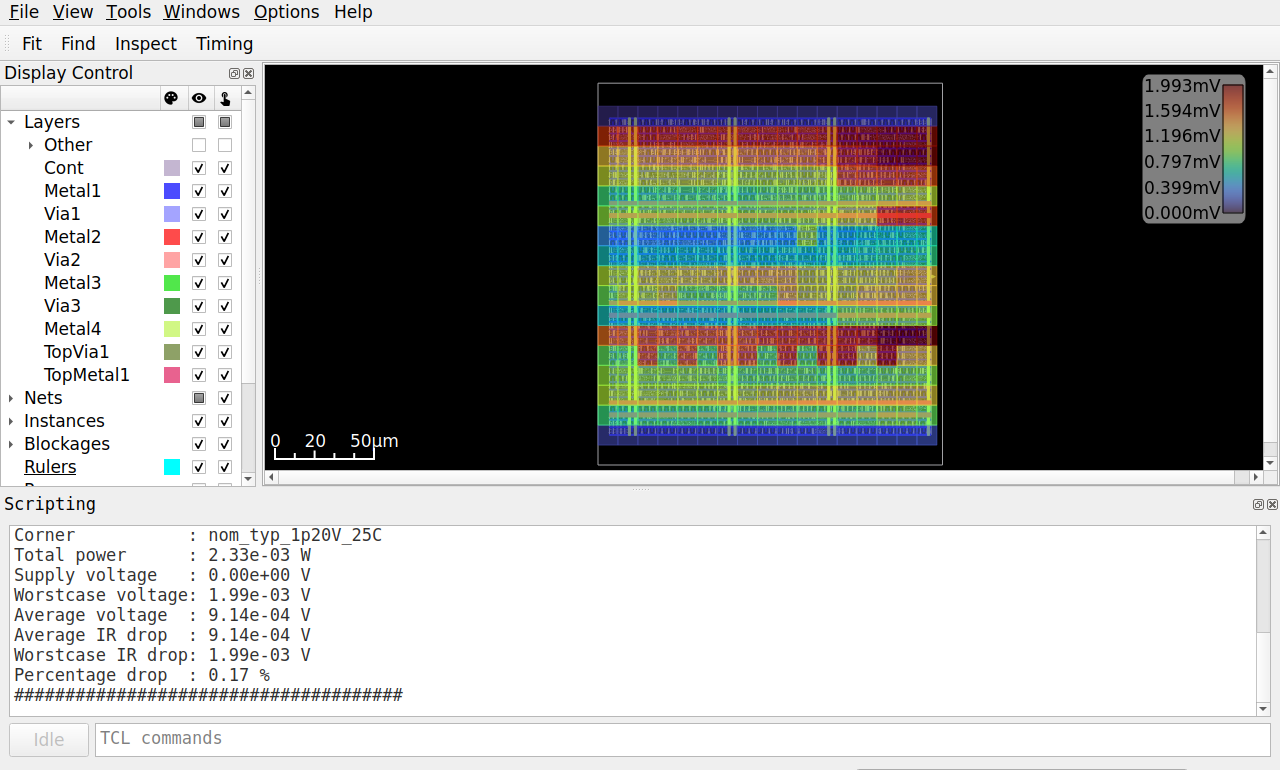
VSS in bs_reg in the OpenROAD GUI after analyze_power_grid -net VSS, with the signal and clock nets hidden.
10.8 Post-Layout Simulation
Signoff STA checks every path, and EQY proves the function of the final netlist, but neither of them runs it. The last simulation does: the testbench of the block on the final netlist, with the delays of the layout. It is the timing simulation of Section 4.10.2, with three differences:
- The wires. The SDF files of the layout hold the delay of every connection from a driver to a load, computed from the extracted parasitics, as
INTERCONNECTentries, 2672 of them forbs_reg. They must stay in the file, and Icarus Verilog annotates them only with the option-ginterconnect. - The clock tree. The clock no longer reaches all flip-flops at once. Each flip-flop sees an edge of
clk_ilate by the delays of the buffers and wires of its path through the tree (Section 10.5), as in STA after CTS. - The corners. LibreLane writes one SDF file per corner into
final/sdf/, e.g.,nom_slow_1p08V_125C/bs_reg__nom_slow_1p08V_125C.sdf, each with the triples of its corner. The option-Tmin,-Ttyp, or-Tmaxofiverilogselects which value of each triple the simulation uses, and-Ttypis the default.
The testbench tb/tb_bs_reg.sv applies random inputs to bs_reg in every cycle and compares data_o with a reference model of the barrel shifter two cycles later. It plays the environment that the SDC of Section 6.6 describes: it changes the inputs 1.0 ns after each rising edge of clk_i, the input delay, and checks data_o 1.0 ns before the next edge, the output delay. Plusargs change the period, the drive and sample times (+DRIVE, +SAMPLE), the number of cycles, and how many mismatches it prints, and +SDF=<file> annotates an SDF file with $sdf_annotate():
bs_reg/tb/tb_bs_reg.sv
// SPDX-FileCopyrightText: 2026 Simon Dorrer
// SPDX-License-Identifier: Apache-2.0
// Description: Testbench of bs_reg for the RTL and the netlist, with
// the delays of an SDF file if +SDF=<file> names one. It changes the
// inputs DRIVE ns after each rising edge and checks data_o SAMPLE ns
// after it, against the inputs of two edges before. Plusargs:
// +PERIOD, +DRIVE, +SAMPLE (ns), +CYCLES, +SHOW (mismatches to
// print), +SDF, +WAVES.

`timescale 1ns / 1ps

module tb_bs_reg;

  real   period = 4.0;  // the clock of the SDC
  real   drive = 1.0;   // the input delay of the SDC
  real   sample = 3.0;  // the period minus the output delay
  int    cycles = 2000, show = 3, errors = 0;
  string sdf;

  logic        clk_i = 1'b0, rst_ni = 1'b0;
  logic [31:0] data_i = '0;
  logic [4:0]  shamt_i = '0;
  logic [1:0]  mode_i = '0;
  logic [31:0] data_o, exp_o, expected [$];

  bs_reg dut (.*);

  // Reference model of the barrel shifter of chapter 4. A rotation
  // shifts two copies of the word side by side.
  function automatic logic [31:0] model(logic [31:0] d,
                                        logic [4:0] s, logic [1:0] m);
    logic [63:0] l, r;
    l = {d, d} << s;
    r = {d, d} >> s;
    case (m)
      2'b00:   model = d << s;
      2'b01:   model = d >> s;
      2'b10:   model = l[63:32];
      default: model = r[31:0];
    endcase
  endfunction

  initial begin
    if ($value$plusargs("SDF=%s", sdf)) $sdf_annotate(sdf, dut);
    void'($value$plusargs("PERIOD=%f", period));
    void'($value$plusargs("DRIVE=%f", drive));
    void'($value$plusargs("SAMPLE=%f", sample));
    void'($value$plusargs("CYCLES=%d", cycles));
    void'($value$plusargs("SHOW=%d", show));
    if ($test$plusargs("WAVES")) begin
      $dumpfile("tb_bs_reg.fst");
      $dumpvars(0, tb_bs_reg);
    end
    #(period / 2);
    forever #(period / 2) clk_i = ~clk_i;  // rising edges at k T
  end

  initial begin
    repeat (2) @(posedge clk_i);
    #(drive) rst_ni = 1'b1;
    for (int k = 0; k < cycles + 2; k++) begin
      @(posedge clk_i);
      #(drive);
      if (k < cycles) begin
        data_i  = $urandom;
        shamt_i = 5'($urandom);
        mode_i  = 2'($urandom);
        expected.push_back(model(data_i, shamt_i, mode_i));
      end
      #(sample - drive);
      if (k >= 2) begin
        exp_o = expected.pop_front();
        if (data_o !== exp_o) begin
          errors++;
          if (errors <= show)
            $display("%0.3f ns: data_o = %h, expected %h",
                     $realtime, data_o, exp_o);
        end
      end
    end
    $display("%0d cycles, %0d errors", cycles, errors);
    $finish;
  end

endmodule
The same testbench runs on the RTL and, with the cell models, on the final netlist without supply connections, final/nl/bs_reg.nl.v. Its decap and fill cells are empty modules in the cell models:
cd /foss/designs/vlsi-design/content/digital_flow/code/bs_reg
iverilog -g2012 -o rtl.vvp \
  ../../../verification/code/barrel_shift/rtl/barrel_shift.sv \
  ../../../sequential/code/bs_reg/rtl/bs_reg.sv tb/tb_bs_reg.sv
vvp -n rtl.vvp
CELLS=$PDK_ROOT/ihp-sg13cmos5l/libs.ref/sg13cmos5l_stdcell/verilog
iverilog -g2012 -gspecify -ginterconnect -o pl.vvp \
  $CELLS/sg13cmos5l_udp.v $CELLS/sg13cmos5l_stdcell.v \
  runs/base/final/nl/bs_reg.nl.v tb/tb_bs_reg.sv
C=nom_typ_1p20V_25C
vvp -n pl.vvp +SDF=runs/base/final/sdf/$C/bs_reg__$C.sdf
Both runs report 2000 cycles, 0 errors. For the RTL, Icarus Verilog warns that it omits $sdf_annotate() without -gspecify, which is harmless there. For the netlist, the compiler prints the 68 sorry messages of Section 4.10.2 and warnings that timing checks are not supported. The simulation prints 71 warnings TIMINGCHECK not supported, one per flip-flop, and two errors Chosen value not defined for the header lines VOLTAGE and TEMPERATURE, whose triples lack the typical value. Unlike the SDF file of Section 4.10.2, the file of LibreLane needs no editing, and all its INTERCONNECT entries are annotated. Icarus Verilog fails on entries from a bit of an input bus that drives several cells, as each bit of data_i in the FIFO does, and here each input bit drives only its input buffer. Without -ginterconnect, each of the 2672 entries gives the error Could not find net, and the simulation runs without the wire delays and still passes. The 2000 cycles take several seconds, a few hundred times as long as the RTL.
As Section 4.10.2 showed, a clean log does not prove that the delays arrived. Check one path: in the waveform, the time from an edge of clk_i to the edge at the clock pin of a flip-flop must equal the sum of the delays along the path in the SDF file, the IOPATH of each buffer and the INTERCONNECT of each wire.
TipExercise: Simulate the Layout
All commands start in the folder content/digital_flow/code/bs_reg and use the run base of the first exercise and the simulations rtl.vvp and pl.vvp compiled above. In a new terminal, define CELLS and C again as above. The instance names and numbers of the solution hold for this run in the image 2026.10, and the testbench draws the same inputs in every run, from the default seed of $urandom.
Sketch the clock path from
clk_ito the flip-flop_1537_ofshamt_q[1], the start of the worst path in the exercise “Close the Timing”. Follow its pinCLKback through the final netlistruns/base/final/nl/bs_reg.nl.v, and write the rising delay of every buffer and every wire from the SDF file of the typical corner next to it. What is the sum? Which delay do you expect in the simulation? Look at thetimescaleof the cell models in$CELLS/sg13cmos5l_stdcell.v.Measure it. The command below writes the waveform
tb_bs_reg.fst, which holds the pins of every cell. Open it withsurfer tb_bs_reg.fstand comparetb_bs_reg.clk_iwithtb_bs_reg.dut._1537_.CLK. When doesCLKof_1537_rise after an edge ofclk_i?vvp -n pl.vvp +SDF=runs/base/final/sdf/$C/bs_reg__$C.sdf \ +CYCLES=10 +WAVES -fstChange the inputs 0.1 ns after each edge instead of 1.0 ns, in the RTL and in the netlist:
vvp -n rtl.vvp +DRIVE=0.1
vvp -n pl.vvp +SDF=runs/base/final/sdf/$C/bs_reg__$C.sdf +DRIVE=0.1
How many cycles fail, by how many cycles is
data_ooff, and what went wrong? Then find the earliest drive time, to 1 ps, at which the netlist still passes in the typical corner. Estimate the limit from the clock path of step 1 and the delay from the inputshamt_i[1]to the pinDof_1537_. Why is the limit a little later than your estimate? What does STA add on top of it?Simulate the slow corner at 4 ns, with the typical values of its SDF file and with the maximum values:
C=nom_slow_1p08V_125C
vvp -n pl.vvp +SDF=runs/base/final/sdf/$C/bs_reg__$C.sdf
iverilog -g2012 -gspecify -ginterconnect -Tmax -o pl_max.vvp \
  $CELLS/sg13cmos5l_udp.v $CELLS/sg13cmos5l_stdcell.v \
  runs/base/final/nl/bs_reg.nl.v tb/tb_bs_reg.sv
vvp -n pl_max.vvp +SDF=runs/base/final/sdf/$C/bs_reg__$C.sdf
Signoff STA failed this corner. How many cycles fail in each simulation? Which flip-flop captures the wrong value, and what is its slack in
runs/base/55-openroad-stapostpnr/nom_slow_1p08V_125C/violator_list.rpt? Then run 20,000 cycles with every mismatch printed (+CYCLES=20000 +SHOW=100). Which bits fail now? Why does the simulation find so few of the endpoints that fail in STA? Compare the data arrival time of each failing path inmax.rptof the corner with the time at which its capture clock edge reaches the flip-flop.
Before continuing, please finish the previous exercise. Once you are done, compare with the solution below.
TipSolution: Simulate the Layout
- The pin
CLKof_1537_hangs on the netclknet_4_10_0_clk_iof the leaf bufferclkbuf_4_10_0_clk_i, which the root bufferclkbuf_0_clk_idrives. In the typical corner, the wire fromclk_ito the root takes 0.002 ns, the rootbuf_80.111 ns, the wire to the leaf 0.013 ns, the leafbuf_80.107 ns, and the wire toCLK0.002 ns, 0.235 ns in all. The cell models declare the timescale1ns/10ps, so Icarus Verilog rounds every cell delay to 10 ps, while the wire delays keep their 1 ps. Both buffers take 0.11 ns, andCLKshould rise 0.22 + 0.017 = 0.237 ns afterclk_i. CLKof_1537_rises exactly 0.237 ns after each rising edge ofclk_i, e.g., at 4.237 ns, and falls 0.236 ns after each falling edge. Every delay along the path is annotated, the wires included.- With
+DRIVE=0.1, the RTL passes, and the netlist fails in 1998 of 2000 cycles.data_oshows each result one cycle early, e.g., at 23 ns,00018f82, the value expected at 27 ns. In the netlist, the clock reaches the input register about 0.24 ns afterclk_i, while the new inputs need only about 0.06 ns to itsDpins. They arrive before the clock edge that the testbench meant for the old values, so the input register takes them one edge too early. In the RTL, every flip-flop samples at the edge ofclk_iitself, so any change after the edge waits for the next one. The netlist passes from a drive time of 0.186 ns on. The estimate from_1537_is 0.237 - 0.055 = 0.182 ns: the rising input takes 0.005 ns on the wire to the input bufferinput37, 0.05 ns in thebuf_1, and nothing on the short wire toD. Of the 39 flip-flops of the input register,_1542_ofmode_q[1]sets the limit: its clock arrives later, at 0.242 ns, and its inputmode_i[1]takes 0.056 ns. At 0.186 ns, the new input reaches itsDin the same picosecond as the clock edge, and the flip-flop still takes the old value. Icarus Verilog takes anyDthat changes beforeCLK, without a hold time or an uncertainty. STA asks for more. Its hold check on the same path takes the latest arrival of the clock, 0.247 ns, adds the uncertainty of 0.1 ns, gets 0.031 ns back from the negative hold time of a fallingD, and compares with the earliest data, 0.060 ns for a falling input. It accepts inputs that change from 0.255 ns on, and in the slow corner from 0.334 ns on. The SDC gives the input delay of 1.0 ns to both the setup and the hold check, so the design was signed off only for inputs that change 1.0 ns after the edge, and only a testbench that keeps to it tests that design. - With the typical values, the slow corner passes all 2000 cycles. With
-Tmax, 3 cycles fail, all in bit 4 ofdata_o, e.g.,aac56072instead ofaac56062at 995 ns. Bit 4 comes from the flip-flop_1508_through the output bufferoutput67, and its slack is -0.504 ns, the second worst in the list after_1516_with -0.586 ns. With 20,000 cycles, 29 cycles fail, 24 in bit 4 and 5 in bit 12, which_1516_drives. In each corner, the typical value of a triple is the mean of the minimum and the maximum, as in Section 4.10.2, and STA checks setup with the maximum. Icarus Verilog checks no setup time and knows no clock uncertainty, so a path can fail only if its data arrives after the capture edge itself. Inmax.rpt, this holds for only 6 of the 31 failing paths: by 0.208 ns for_1516_, by 0.191 ns for_1508_, and by less than 0.1 ns for four more. The other 25 fail in STA only through the setup time and the uncertainty, so no stimulus can make them fail in this simulation. The six fail only in the cycles in which the stimulus causes their slowest transitions, and in 20,000 cycles, the simulation finds the two worst of them, with the typical values none. Signoff rests on STA. The post-layout simulation checks what STA takes from the SDC on trust: that the testbench, or the block outside, behaves like the environment the SDC describes, and that the netlist with all its delays still computes the right function.
10.9 Chip Assembly
A macro is not yet a chip. The chip top level of the AMS chip template (Section 1.10) places the macros into a core and surrounds it with a padframe: a ring of IO cells, each with its bondpad, which drive the signals off the chip, protect the inputs against electrostatic discharge, and bring in the supplies (Figure 71). It runs LibreLane’s Chip flow, the Classic flow with additional steps: one builds the padframe, one draws the seal ring, a wall of all metal and via layers along the edge of the die that stops cracks from the sawing and keeps moisture out, and two insert the fill and check its density. In its configuration, flow/librelane/config.yaml of the template:
- The die is 1.6 mm × 1.6 mm, with the core from 365 to 1235 µm in both directions, and the clock is 20 ns.
- Four lists,
PAD_WEST,PAD_NORTH,PAD_SOUTH, andPAD_EAST, name the 32 pad instances of the RTL in the order in which they line up on each side: inputs, outputs, bidirectional pads with the tri-state drivers of Section 3.4.4, analog pads, and the supply pads for the core (VDD,VSS, 1.5 V) and for the IO cells (IOVDD,IOVSS, 3.3 V). - The timing is signed off for both core supplies of the PDK, in the typical, slow, and fast corners at 1.2 V and at 1.5 V, with the typical corner at 1.5 V as the default.
- The block
MACROSlists each macro with its GDSII and LEF and, where they exist, its netlists, parasitics, and timing models per corner, and places its instances at fixed positions and orientations.PDN_MACRO_CONNECTIONSconnects the two supply pairs of the SRAM to the grid of the core, and the other macros get their supplies through their power pins in the RTL. - A core ring of 15 µm wide supply wires surrounds the core and connects to the supply pads (
PDN_CORE_RING_CONNECT_TO_PADS). - A non-default routing rule gives the analog nets wires of 0.5 µm width and spacing on Metal1 to Metal4, and the resizer must not touch them.
The template switches off the fill step of the flow. After the run, it adds the chip logo and then the fill, which brings the density of the active area and of every metal layer into the window that manufacturing demands, e.g., 35 to 60 % on Metal1 to Metal4, checks the whole chip with the DRC of Magic (KLayout runs its DRC and LVS with make klayout-drc and make klayout-lvs), and draws the bonding diagram for the package. Section 11 builds a chip this way.
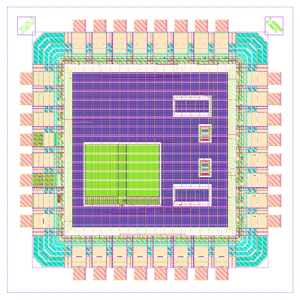
The Makefiles of the template wrap the GUI and the reports in two targets, for the chip and for each macro. make librelane-openroad opens the last run with --last-run --flow OpenInOpenROAD, i.e., the run that changed last, and make copy-reports copies the most important reports of the run into the repository, to verification/reports/ of the chip and to verification/ of a macro. At the top level, a macro is a black box with pins and a timing model. In the Clock Tree Viewer of the template chip (Figure 72), the clock from its pad passes three clock buffers and reaches only three sinks, the two counters and the SRAM. Each counter appears as a bar from its clock pin, as long as the clock latency inside it, which its timing model gives (max_clock_tree_path, about 0.1 ns). The SRAM, whose timing model gives none, is a short box. The timing model that LibreLane writes for a hardened macro, final/lib/ of the counter, holds no power at all, though. The power report of the chip counts such a macro with 0 W, and the IR drop analysis of the chip, which takes its currents from these numbers, misses all of its current. The signoff of a hardened macro therefore stays in its own run.
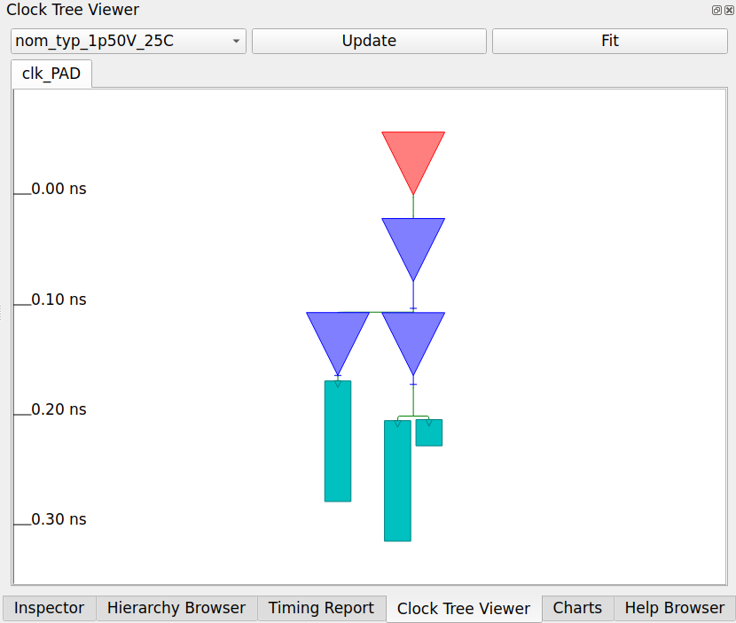
10.9.1 Static Cells and PCells
Most of this chip consists of static cells, layouts with fixed geometry. The standard cells, the IO cells, and the SRAM macros come as GDSII files with the PDK (Section 5.3.1), and a macro hardened by LibreLane is a static cell as well. A different size is a different cell, e.g., inv_1 and inv_4. In return, a fixed layout has to be characterized only once per corner, so a library can describe each cell with one LEF abstract and its Liberty tables.
The bondpad and the seal ring, in contrast, come from parameterized cells (PCells). A PCell is a small program that draws a layout from parameters. For example, the PCell nmos with w=10u, l=0.13u, and ng=4 draws the active area, four gate fingers of 2.5 µm width each, and the contacts of source and drain. This suits analog layout, where devices come in many sizes. The PCells of SG13CMOS5L are Python code in the PDK (libs.tech/klayout/python), and KLayout offers them in the library SG13_dev, e.g., nmos, rhigh, via_stack, bondpad, and sealring. In the template, make build-bondpad runs the bondpad PCell for a square pad of 70 µm × 70 µm, and the step KLayout.SealRing draws the sealring PCell for the size of the die, so that the ring fits any chip.
A PCell exists only in the layout tool, because GDSII stores only polygons, paths, texts, and cell references. Saving a layout writes each parameter set as an ordinary cell. KLayout can also store the parameters in the file, and when it reads such a file with the PDK installed, it redraws the PCells. This keeps the devices editable, but after a PDK update, the same file can yield different geometry. A layout for tapeout is exported without the parameters, so every PCell becomes a static cell and the geometry stays fixed. The export itself redraws the PCells with the installed PDK, so DRC and LVS have to run on the exported file. The inverter macro of the template keeps both files in macros/inverter/layout: inverter_top.klay.gds for editing and inverter_top.gds, written with File > Export Layout For Tapeout, for the flow.
10.10 Summary
- LibreLane runs the flow as a list of steps, each with its own folder of logs and reports in the run folder, and collects GDSII, LEF, netlists, SPEF, SDF, and metrics in
final/. A YAML file sets what the defaults of LibreLane and the PDK do not. - The flow
OpenInOpenROADopens a run in the OpenROAD GUI, with the timing of the default corner only, and an earlier state under a run tag of its own. The Clock Tree Viewer shows when the clock edge reaches each buffer and flip-flop, the heat maps show the routing congestion after global routing and the IR drop afteranalyze_power_grid, and the Timing Report draws the worst paths into the layout. - The floorplan sizes the core from the cell area and a utilization, divides it into rows of 3.78 µm, and builds the power grid from Metal1 rails and Metal4 and TopMetal1 straps.
- Placement spreads the cells and buffers every net beyond the limits of slew, capacitance, and fanout, e.g., the reset net. CTS builds an H-tree of
buf_8with a small skew and balances clock gates, but not divided clocks. The timing repair fixes setup and hold with the propagated clock. - Routing assigns and draws every wire, repairs antenna violations, and fill insertion adds decaps and fillers.
- Signoff extracts the wires and checks the timing in all corners, the IR drop, the design rules, and the layout against the netlist. EQY then proves the final netlist equivalent to the RTL. The estimates before routing are optimistic, so the repair needs a margin, and in
bs_regthe slow corner passes with a setup margin of 0.6 ns. Flow complete.does not mean a clean design: the setup checker counts only the typical corners, andmanufacturability.rptcovers antenna, LVS, and DRC only. Read the timing, the limits, the power, and the IR drop in the reports of the run (Section 10.7.1).- The post-layout simulation compiles the final netlist with
-gspecify -ginterconnectand runs the testbench with the SDF file of one corner. Check one path against the SDF file to prove the annotation, and drive the inputs and sample the outputs as the SDC describes, because the clock tree delays the clock edge at every flip-flop. Without timing checks, it finds only paths whose data arrives after the clock edge, and only when its stimulus triggers them, so signoff rests on STA. - The chip top level of the AMS chip template runs LibreLane’s Chip flow, which places the macros in a core inside a padframe of IO cells and bondpads and draws the seal ring. At the top level, a hardened macro is a black box with a timing model that holds its clock latency but no power, so its signoff stays in its own run.
- The cells of the PDK’s libraries and hardened macros are static cells with fixed geometry. A PCell draws a layout from parameters, e.g., the bondpad and the seal ring, and a layout for tapeout is exported as static cells.
In Section 11, these steps build a complete chip with the AMS chip template.
11 Capstone Project: A Small RISC-V SoC
Note
This chapter will be released later in the semester.
12 Appendix: Exam Questions
This appendix collects possible questions for the written exam (Section 1.5), grouped by the chapters of the course. The last two sections hold calculation problems and problems in which you read, write, or fix code, constraints, and reports. The exam is based on these questions, partly with other numbers, circuits, or code.
The written exam is closed book and allows no technical aids. Most questions therefore ask for an explanation, often with a sketch, and the calculations need only simple arithmetic, with every value and constant given in the question. If you have worked through the exercises of the chapters, you have practiced most of what these questions ask. The practical work with the tools is assessed in the project (Section 11).
12.1 Introduction
Compare the ASIC implementation styles FPGA, gate array, standard-cell IC, and full-custom IC by the masks they need, the design effort, the trade-off between non-recurring engineering cost and unit cost, and their typical use. Which style does this course use, and what does the designer describe in it?
Draw the RTL-to-GDSII flow from the RTL to the tapeout, and explain each step in one sentence. Where does a design iteration go back to when the timing is not met?
12.2 Hardware Description with SystemVerilog
How does a hardware description differ from a program for a microcontroller? Use a
forloop to explain computing in time and computing in space, and what happens to the run time and the area when the loop bound grows.How does SystemVerilog extend and truncate the operands of an expression? Give an example in which a carry is lost without a warning and one in which a comparison with a constant is always false. How do you keep the carry, and what happens when signed and unsigned operands are mixed?
Explain the difference between the blocking assignment
=and the non-blocking assignment<=. What happens when two registers that should swap their values are written with blocking assignments in onealways_ffblock, and what happens when the two blocking assignments sit in two separatealways_ffblocks? State the golden rules of processes.Explain the two-process style in SystemVerilog. What belongs in the
always_ffblock and what in thealways_combblock, what do the suffixes_dand_qstand for, and which advantages does the style have?When does a combinational block infer a latch, and why is an unintended latch almost always a bug in a synchronous design? How does a default assignment prevent it, and what do Verilator and Yosys report for a latch in
always_comb? Is a register that keeps its value while its clock enable is low a latch?What is the difference between a Moore and a Mealy FSM? A controller raises
done_ofor one clock cycle when a job ends. Compare a Moore and a Mealy version by the number of states, the cycle in whichdone_ois high, and the risks of the output.What makes a testbench self-checking? Why does a testbench drive the inputs and check the outputs on the falling clock edge? How must a failing check end an Icarus Verilog simulation, and what must the runner of a cocotb testbench do, so that a script sees the failure?
12.3 Modeling Guidelines for Synthesizable RTL
Why must the simulation of the RTL agree with that of the netlist, and what are the typical causes of a mismatch? What can a gate-level simulation see that a logic equivalence check cannot, and the other way round?
What do X-optimism and X-pessimism mean? How do an
if, acasewhosedefaultassigns'x, and the conditional operator?:treat an unknown select in Icarus Verilog, and how does an AND gate treat an unknown input? Why does Verilator show noxat all, and why should RTL never assign'x?Which registers need a reset, and which may stay without one? Why can the missing reset of an FSM stay invisible in an RTL simulation, and which simulations reveal it?
Name four habits from FPGA design that break on an ASIC, and what you use instead. Why in particular is a register output that clocks other registers a problem, and how does a clock enable avoid it?
An exclusive counter can be built as a binary counter with a decoder, as a one-hot ring, or as a Johnson counter with a decoder. Compare the three architectures by area, speed, glitches at the outputs, and robustness against a wrong state. Does the coding style, e.g., a
forloop instead of a concatenation for the ring, change the netlist?
12.4 Functional Verification with cocotb
Distinguish verification, test, and validation. What does each of them ask, and when does it happen? What is the fundamental limit of simulation?
Draw a testbench with generator, driver, monitor, reference model, scoreboard, and coverage collector, and explain each block. Why is the reference model written from the specification and not from the RTL, and which blocks merge for a combinational design?
Compare directed, exhaustive, and constrained-random stimuli, and explain how you reproduce a random test that failed. Why can an exhaustive test of the 8-bit instance of a parameterized barrel shifter miss a bug of its 32-bit instance?
Name the four kinds of code coverage that Verilator measures. What is functional coverage, and how can a test reach 100 % line, branch, and expression coverage while it misses most of the functional bins? What does no kind of coverage measure?
What is the difference between an immediate and a concurrent assertion? Explain
|->,|=>,disable iff, and$stable(). Why are the concurrent assertions of the course kept in a separate checker attached withbind?What is mutation testing? Explain killed, surviving, and equivalent mutants, and the two possible reasons why a mutant survives.
What does an SDF file hold, and what does back-annotation mean? Why can a timing simulation with Icarus Verilog pass at clock periods for which static timing analysis reports violations, and which of the two do you trust for the tapeout? Why can Verilator not run this simulation, and for which tasks do you choose it over Icarus Verilog?
12.5 Logic Synthesis and the Standard-Cell Library
Describe the four steps of logic synthesis from the RTL to a netlist of standard cells. Which Yosys commands perform them?
What is a standard cell? Explain rows, sites, shared supply rails, and the drive strength of a cell, and name the views of a standard-cell library with the steps of the flow that read them.
What information does a Liberty file hold for a cell? Explain a timing arc and its timing sense, with an example of a positive unate, a negative unate, and a non-unate arc. Between which points of the waveforms are a delay and a slew measured?
What is the propagation delay of a cell, and what does it depend on? How does the nonlinear delay model store it, how does a timing tool compute the delay between the table entries, and why is the delay of a path computed stage by stage?
What is a wire-load model, from what does it estimate the capacitance of a wire, and when is it used? Which wire capacitances do the pre-layout timing analyses of this book include?
What are process, voltage, and temperature corners? Which corner usually limits the setup check and which the hold check, and why does the signoff check both in all corners?
What does a logic equivalence check prove, and why does a netlist need one, although synthesis produced it from the RTL? Explain gold, gate, the matching of registers, cut points, and cones, and name two cases in which the check fails falsely.
An equivalence check fails in one partition. How do you decide whether the netlist has a bug or the check failed falsely, and why should a check that passes also be shown to fail on a broken netlist?
12.6 Sequential Elements and Static Timing Analysis
What are the setup time and the hold time of a flip-flop, and what can happen when the data changes inside the window that they form? Name the other timing parameters of a flip-flop with an asynchronous reset, and explain what a negative hold time means.
Draw a path between two registers with the clock tree that drives both. What are clock latency, clock skew, clock uncertainty, and jitter?
Write the setup and the hold condition of a register-to-register path, including skew and uncertainty, and define the slack of each check. Describe a setup and a hold violation. Why does a lower clock frequency fix a setup violation but not a hold violation?
Describe static timing analysis in one sentence. What are startpoints, endpoints, and the four kinds of timing paths, and what are WNS and TNS? What can static timing analysis not check?
A register output clocks other registers. What does STA do with the paths behind it if the constraints do not mention this clock, and how does
check_setupreveal it? Which constraint fixes the analysis, and which paths does the tool time once it knows the generated clock?What are false paths and multicycle paths? Why does a multicycle path with 2 cycles for setup also need an exception of 1 cycle for hold? Why should a design have few timing exceptions?
How are setup and hold violations fixed, and on which paths do hold violations typically appear? The capturing flip-flop of a shift register of two flip-flops gets its clock through four buffers, and the analysis uses no clock uncertainty. Why can its hold check be worst in the slow corner?
12.7 Synthesis Optimizations and Low-Power Design
Explain the generate and the propagate signal of an adder, its carry recursion, and the prefix operator. Compare the ripple-carry, Brent-Kung, and Kogge-Stone adders by the number of levels and of prefix operators, and draw the prefix graph of an 8-bit Kogge-Stone adder.
A prefix adder written with
+comes out of synthesis with almost as many gates on its worst path as a ripple-carry adder. Why, and what follows for writing arithmetic in RTL?Why does a pipeline raise the throughput but not shorten the latency, and what limits the gain of more stages? Which signals must pass through the pipeline as well? What is retiming, and why does it complicate the equivalence check?
Name the three components of the power consumption of a CMOS circuit, and write the formula of the switching power. Which levers reduce the dynamic and the static power, and why does a slower clock alone not save energy per operation?
Why does a plain AND gate of the clock and an enable not work as a clock gate? Draw an integrated clock gate and its waveforms, and explain why it uses a latch. Why does clock gating save most of the power of a register whose enable is rarely high, but little when the enable is high in every cycle?
12.8 Clock Domains, Metastability, and Resets
What is a clock domain, and when are two clocks synchronous or asynchronous? What is a clock domain crossing, why can static timing analysis not check it, and which SDC command removes the paths between two asynchronous clocks from the analysis?
Explain metastability with the cross-coupled inverters of a latch and its time constant \(\tau\). Write the formula for the mean time between failures (MTBF) of a synchronizer, explain each term, and say why a synchronizer is designed for the slow corner.
Draw a two-flip-flop synchronizer and explain why it raises the MTBF. Which rules must a synchronizer follow, and by which factor does a third flip-flop raise the MTBF?
Why can a one-cycle pulse from a fast clock domain get lost in a slow one? Draw a pulse synchronizer and explain how it works. How far apart must two pulses be?
Why can a bus whose bits change at the same time not cross through one synchronizer per bit? Name three ways to cross it, explain why Gray code works for counters and pointers, and describe a handshake.
Draw an asynchronous FIFO. Why does each pointer exist in binary and in Gray code? How are the full and the empty flag computed, why can they be pessimistic, and why does the memory need no synchronizer?
Why is the release of an asynchronous reset a clock domain crossing? What does a reset synchronizer do, how many does a design with several clock domains need, and why must the reset input itself be free of glitches?
12.9 Design for Test (DFT)
Why must every manufactured die be tested, and how do catastrophic and parametric yield loss differ? Name the three tests that a die can go through between the wafer and the shipment, and what each of them catches. Sketch the bathtub curve of the failure rate, and explain with it what a burn-in does.
What are yield, fault coverage, test coverage, and defect level? Write the model of Williams and Brown, and explain why a defect level of a few ppm needs a fault coverage close to 100 %. What is overkill, and what does it cost?
Explain the chain of defect, fault, error, and failure. What is the stuck-at fault model, and what are the stem and the branches of a net? How many single stuck-at faults does a netlist with \(n\) fault sites have? What are equivalent and untestable faults, and what does fault collapsing do?
Name three kinds of production defects, the wrong behavior that each of them causes, and the fault model that describes it. Why does a stuck-open transistor need a test of two vectors, and why can a stuck-on transistor escape every test of the logic values? What does IDDQ testing measure?
Describe the three steps of finding a test for a stuck-at fault, and explain controllability and observability. What do the values \(D\) and \(\bar{D}\) of the D-algorithm stand for, and what are the D-frontier and the J-frontier? How does PODEM differ from the D-algorithm? How do the D-algorithm and a SAT solver on a miter show that a fault is untestable, and why do ATPG tools start with random vectors?
What is scan design? Draw a scan flip-flop and a scan chain, and explain how scan turns the test of a sequential circuit into the test of a combinational one. What does scan cost, why are the chains stitched only after the placement, and how do you check that the scan insertion did not change the function?
Describe the scan test sequence, including the chain test. How many clock cycles does a test of \(N\) patterns over a chain of \(L\) flip-flops take, and how can the test time be reduced? Why is the shift clock often slower than the functional clock?
Name and explain at least four design rules for testability besides those for the scan chain itself. Why does a reset synchronizer in front of the registers break the scan chain, and how is it fixed?
What do an at-speed test, a logic built-in self-test, a memory BIST, and boundary scan add to the scan test? Explain launch on capture, launch on shift, and aliasing. Why should a transition test sensitize the longest path through a fault site?
12.10 The RTL-to-GDSII Flow with LibreLane
What are the die and the core of a floorplan? How does the utilization set the size of the core, and why is the core not filled with cells completely? How are the rows, the power grid, and the pins arranged, and what does a denser core gain and cost?
What do global placement, the repair of the design, and detailed placement do? Which limits does the repair of the design enforce, what happens to the timing of a net that exceeds them, and why does the reset net need the repair?
What is a clock tree, and what is it used for? How does TritonCTS build an H-tree, and what is a dummy load?
What changes in the timing analysis after clock tree synthesis, and why does the flow repair hold violations only after it? How does CTS treat a clock gate, and why do the paths into a divided clock violate hold?
What do global and detailed routing do, and what is congestion? What is the antenna rule, and how is a violation fixed? Which cells does the fill insertion add to the rows after routing, and why?
What does the signoff check? Explain parasitic extraction, the signoff STA in all corners, the IR drop analysis, DRC, and LVS, and say why the equivalence check runs again on the final netlist.
How does the flow estimate the wires after placement, and why are these estimates optimistic? Why does the slow corner lose the most slack, and why can a setup margin for the timing repair close the timing where a delay-oriented synthesis does not?
What changes when a timing simulation runs on the final netlist after the layout instead of on the synthesized netlist, and how do you check that the delays of the SDF file were really annotated? Why must the testbench change the inputs no earlier than the input delay of the SDC, and what happens in the simulation when it changes them right after the clock edge?
What does a padframe do? What do the IO cells, the core ring, the seal ring, and the metal fill add to a chip, and which steps does the Chip flow add to the Classic flow?
What is the difference between a static cell and a PCell? Give an example of each, and say what happens to a PCell when a layout is exported for tapeout.
12.11 Calculation Problems
Delay Table: Around an input slew of 0.2 ns and a load of 0.03 pF, the table
cell_riseof a cell holds four entries: 0.10 ns at a slew of 0.1 ns and a load of 0.02 pF, 0.20 ns at 0.1 ns and 0.06 pF, 0.14 ns at 0.3 ns and 0.02 pF, and 0.26 ns at 0.3 ns and 0.06 pF. Compute the delay by linear interpolation, first along the load and then along the slew.Setup and Hold Slack: A path between two flip-flops on the same clock has a clock-to-output delay of 0.2 ns, a longest logic delay of 1.5 ns, a shortest logic delay of 0.02 ns, a setup time of 0.1 ns, and a hold time of 0.05 ns. The clock reaches the capturing flip-flop 0.1 ns later than the launching one, and the clock uncertainty is 0.1 ns for both checks. Compute the setup slack at a clock period of 2 ns, the minimum period, and the hold slack. Which check fails, does a slower clock help, and how do you fix it?
Switching Power: The data nets of a block have a total capacitance of 20 pF and an average activity of 0.1 transitions per clock cycle, and its clock net has 2 pF. Compute the switching power of the data nets and of the clock net at 1.2 V and 250 MHz. By which factor does the switching power grow at 1.5 V and the same clock frequency?
Synchronizer MTBF: A flip-flop has \(\tau\) = 100 ps and \(T_0\) = 20 ps, a clock-to-output delay of 0.2 ns, and a setup time of 0.1 ns. A signal that changes \(10^7\) times per second enters a domain clocked at 500 MHz through a two-flip-flop synchronizer. Compute the MTBF, the factor by which a third flip-flop raises it, and the MTBF with three flip-flops in years. Use \(e^{17} \approx 2.4 \cdot 10^7\) and 1 year \(\approx 3.2 \cdot 10^7\) s.
Defect Level: A process has a yield of 90 %, and the test reaches a fault coverage of 98 %. Compute the defect level in ppm with the model of Williams and Brown, and the coverage that a defect level of 10 ppm needs. Use \(Y^x \approx 1 + x \ln Y\) for small \(x\), and \(\ln 0.9 \approx -0.105\).
Test Vectors: A circuit computes \(y = ab + c\), with the internal net \(n = ab\). Find a test vector \((a, b, c)\) for \(n\) stuck-at-0, for \(a\) stuck-at-1, and for \(c\) stuck-at-0, and say for each how it excites and propagates the fault, with the values \(D\) and \(\bar{D}\) along the path. Then show with the D-algorithm that the net \(bc\) stuck-at-0 in \(y = ab + \bar{a}c + bc\) is untestable.
Scan Test Time: A design has 1000 flip-flops, and its test has 200 scan patterns, which the tester shifts at 20 MHz. How long does the scan test take without the chain test, with one chain, and how long with 10 chains of 100 flip-flops each?
Fault Collapsing: A circuit has the inputs \(a\), \(b\), \(c\), and \(d\) and two outputs. An AND gate computes \(p = ab\), an OR gate \(y = p + c\), an inverter \(\bar{c}\), and a second AND gate \(z = \bar{c}\,d\), so \(c\) drives the OR gate and the inverter. Count the fault sites with a site on each net and on each branch of \(c\), and the single stuck-at faults. How many faults does the rule \(2(P_O + F_O) + G_I - N_I\) leave? Which faults are equivalent to \(y\) stuck-at-1, and which to \(z\) stuck-at-0?
Delay Test: A net lies on two paths between flip-flops of the same clock, with delays of 1.2 ns and 1.9 ns, each including the clock-to-output delay and the setup time. The clock is ideal and has no uncertainty. A defect adds an extra delay to the net. Which extra delay must the defect exceed, so that an at-speed transition test at the functional clock period of 2 ns detects it along each of the two paths? Which path should the test use? Which extra delay must the defect exceed for the better path if the test runs with a slow test clock of 4 ns instead?
Gray Code: Write down the 3-bit Gray code of 0 to 7. Convert the binary value
1011into Gray code, and the Gray code1101back into binary. A 4-bit binary counter steps from0111to1000while another clock domain samples it through one synchronizer per bit. Which values can the other domain see, and which with a Gray-coded counter?
12.12 Reading, Writing, and Fixing Code
Find the Bugs: The following module should add
d_ito an 8-bit sum in every clock cycle in whichen_iis high and keep the sum otherwise. The sum wraps around at 256. Find the three mistakes. For each one, explain what Verilator or Yosys reports or which hardware results, and write the corrected module.module acc ( input logic clk_i, input logic rst_ni, input logic en_i, input logic [7:0] d_i, output logic [7:0] sum_o ); logic [7:0] sum_d, sum_q; always_ff @(posedge clk_i or negedge rst_ni) begin if (!rst_ni) sum_q = '0; else sum_q = sum_d; end always_comb begin if (en_i) sum_d = sum_q + d_i; end assign sum = sum_q; endmoduleFrom VHDL to SystemVerilog: The following counter is written in the two-process style of VHDL, with
cntandnext_cntof typeunsigned(2 downto 0). Translate it into a SystemVerilog modulecnt3with the portsclk_i,rst_ni,en_i,clr_i, andtc_o, an asynchronous active-low reset, and the two-process style with_dand_q. Why must the sensitivity list ofcnt_logiccontain all three signals, and what replaces it in SystemVerilog?reg_proc: process(rst_i, clk_i) is begin if rst_i = '1' then cnt <= (others => '0'); elsif rising_edge(clk_i) then cnt <= next_cnt; end if; end process reg_proc; cnt_logic: process(cnt, en_i, clr_i) is begin next_cnt <= cnt; if clr_i = '1' then next_cnt <= (others => '0'); elsif en_i = '1' then next_cnt <= cnt + 1; end if; end process cnt_logic; tc_o <= '1' when cnt = 7 else '0';Clock Enable Instead of a Divided Clock: The following code counts at half the clock frequency. Rewrite it with only one clock, an asynchronous active-low reset
rst_ni, and a clock enable, so that the counter still advances at every second rising edge ofclk_i. What does a simulation of the original with Icarus Verilog show, sincediv_qhas no reset, and why does your version not have this problem?always_ff @(posedge clk_i) begin div_q <= ~div_q; end always_ff @(posedge div_q) begin cnt_q <= cnt_q + 1'b1; endLiberty Cell: The following excerpt describes a cell of the typical library, whose units are ns and pF.
cell (sg13cmos5l_a21oi_1) {
  area : 9.072;
  pin (Y) {
    direction : "output";
    function : "!((A1*A2)+B1)";
    max_capacitance : 0.3;
    timing () {
      related_pin : "A1";
      timing_sense : negative_unate;
      timing_type : combinational;
      cell_rise (TIMING_DELAY_7x7ds1) { ... }
      cell_fall (TIMING_DELAY_7x7ds1) { ... }
    }
  }
  pin (A1) {
    direction : "input";
    capacitance : 0.00301392;
  }
}
Draw the gate that the function describes. What does the timing sense of the arc from
A1toYmean? How large is the cell in gate equivalents, if a 2-input NAND gate has 7.2576 µm²? What is the input capacitance ofA1in fF, and what happens when the output has to drive more thanmax_capacitance?Timing Report: The following report of OpenSTA shows the worst setup path of a block with an ideal clock of 1.25 ns.
Startpoint: a_q (rising edge-triggered flip-flop clocked by clk)
Endpoint: b_q (rising edge-triggered flip-flop clocked by clk)
Path Group: clk
Path Type: max

  Delay    Time   Description
-----------------------------------------------------------
  0.000   0.000   clock clk (rise edge)
  0.000   0.000   clock network delay (ideal)
  0.000   0.000 ^ a_q/CLK (sg13cmos5l_dfrbpq_1)
  0.210   0.210 v a_q/Q (sg13cmos5l_dfrbpq_1)
  0.650   0.860 ^ u1/Y (sg13cmos5l_nor4_1)
  0.290   1.150 ^ u2/X (sg13cmos5l_mux2_1)
  0.000   1.150 ^ b_q/D (sg13cmos5l_dfrbpq_1)
          1.150   data arrival time

  1.250   1.250   clock clk (rise edge)
  0.000   1.250   clock network delay (ideal)
 -0.100   1.150   clock uncertainty
  0.000   1.150   clock reconvergence pessimism
          1.150 ^ b_q/CLK (sg13cmos5l_dfrbpq_1)
 -0.120   1.030   library setup time
          1.030   data required time
-----------------------------------------------------------
          1.030   data required time
         -1.150   data arrival time
-----------------------------------------------------------
         -0.120   slack (VIOLATED)
Is the check met? Compute the minimum clock period of this path. Which cell takes the most time, and why is its rising output slow? Propose two fixes. Which lines of the two clock paths change if only
set_propagated_clockis added to the constraints after clock tree synthesis, and why?Timing Constraints: Write the SDC constraints for a block with the clock input
clk_iat 200 MHz, a clock transition of 0.1 ns, a clock uncertainty of 0.15 ns, input delays of 1.5 ns at all other inputs, output delays of 1.5 ns at all outputs, the cellsg13cmos5l_buf_2with its output pinXas the driver of the inputs, and a load of 10 fF at the outputs, in the units of the library, ns and pF. Explain what each command tells the timing analysis.Clock Domain Crossing:
req_ais a pulse of one cycle of the faster clockclk_a_i, and the following code takes it into the domain ofclk_b_i. Find the three mistakes, and draw a corrected crossing.// domain A assign req_a = start_a_i & ready_a_q; // domain B always_ff @(posedge clk_b_i or negedge rst_b_ni) begin if (!rst_b_ni) begin s1_q <= 1'b0; s2_q <= 1'b0; end else begin s1_q <= req_a; s2_q <= s1_q & en_b_i; end end
References
Bergeron, Janick. 2006. Writing Testbenches Using SystemVerilog. Springer.
Brayton, Robert, and Alan Mishchenko. 2010. “ABC: An Academic Industrial-Strength Verification Tool.” Computer Aided Verification (CAV 2010), Lecture notes in computer science, vol. 6174: 24–40.
Bushnell, Michael L., and Vishwani D. Agrawal. 2000. Essentials of Electronic Testing for Digital, Memory and Mixed-Signal VLSI Circuits. Kluwer Academic Publishers.
Castañeda, Oscar, Lavinia Recchioni, Tobias Senti, et al. 2026. An Open-Source Standard-Cell Library for IHP 130 nm Developed by Students. arXiv preprint 2609.29965, https://arxiv.org/abs/2609.29965.
cocotb developers. 2026. cocotb: A Coroutine-Based Cosimulation Testbench Environment for Verifying VHDL and SystemVerilog RTL Using Python. Https://github.com/cocotb/cocotb.
Cummings, Clifford E. 2002. “Simulation and Synthesis Techniques for Asynchronous FIFO Design.” SNUG San Jose.
Cummings, Clifford E. 2008. “Clock Domain Crossing (CDC) Design & Verification Techniques Using SystemVerilog.” SNUG Boston.
Dorrer, Simon. 2025. “An Open-Source Adaptive Event-Based ADC for Bio-Signal Acquisition in 130 nm CMOS.” Master’s thesis, Johannes Kepler University Linz. https://epub.jku.at/urn/urn:nbn:at:at-ubl:1-90281.
Dorrer, Simon, and Harald Pretl. 2026. An Open-Source Analog Mixed-Signal Chip Design Template & Tutorial for the ihp-sg13cmos5l Open-PDK. Https://github.com/iic-jku/ihp-sg13cmos5l-ams-chip-template. https://doi.org/10.5281/zenodo.22115134.
Freitas, Édney M. V., Nicolas Guimarães, Rafael Maria, et al. 2025. “Using Open Source EDA Tools in ASICs for HEP: A Mixed Comparison.” Journal of Instrumentation 20 (12): P12022. https://doi.org/10.1088/1748-0221/20/12/P12022.
Gaber, Mohamed. 2026. Difetto: A Novel Design-for-Test Flow Using LibreLane. Https://github.com/donn/difetto.
Goel, Prabhakar. 1981. “An Implicit Enumeration Algorithm to Generate Tests for Combinational Logic Circuits.” IEEE Transactions on Computers C-30 (3): 215–22.
Harris, Sarah L., and David Money Harris. 2021. Digital Design and Computer Architecture, RISC-V Edition. Morgan Kaufmann.
IEEE. 2001. IEEE Standard for Standard Delay Format (SDF) for the Electronic Design Process.
IEEE. 2020. IEEE Standard for Universal Verification Methodology Language Reference Manual.
IEEE. 2024. IEEE Standard for SystemVerilog: Unified Hardware Design, Specification, and Verification Language. https://doi.org/10.1109/IEEESTD.2024.10458102.
Institute for Integrated Circuits and Quantum Computing, JKU. 2026. IIC-OSIC-TOOLS: A Container with Open-Source IC Design Tools. Https://github.com/iic-jku/IIC-OSIC-TOOLS.
LibreLane Project. 2026. LibreLane: An Open-Source Digital RTL-to-GDSII Flow. Https://github.com/librelane/librelane.
lowRISC. 2026. lowRISC Verilog Coding Style Guide. Https://github.com/lowRISC/style-guides/blob/master/VerilogCodingStyle.md.
OpenCDC developers. 2026. OpenCDC: Static Clock Domain Crossing Analyzer for Verilog and SystemVerilog. Https://github.com/Ayoubbelguellaoui/CDC.
Parallax Software, and The OpenROAD Project. 2026. OpenSTA: Static Timing Analyzer. Https://github.com/The-OpenROAD-Project/OpenSTA.
Popoloski, Mike. 2026. slang: SystemVerilog Language Services. Https://github.com/MikePopoloski/slang.
pyuvm developers. 2026. pyuvm: The Universal Verification Methodology in Python. Https://github.com/pyuvm/pyuvm.
Roth, J. Paul. 1966. “Diagnosis of Automata Failures: A Calculus and a Method.” IBM Journal of Research and Development 10 (4): 278–91.
Sánchez Lopera, Daniela, Sven Wenzek, and Wolfgang Ecker. 2022. “Using Open-Source EDA Tools in an Industrial Design Flow.” Design and Verification Conference and Exhibition Europe (DVCon Europe). https://dvcon-proceedings.org/wp-content/uploads/74522.pdf.
Smith, Gordon L. 1985. “Model for Delay Faults Based Upon Paths.” Proceedings of the International Test Conference (ITC), 342–49.
Snyder, Wilson et al. 2026. Verilator: SystemVerilog Simulator and Lint Tool. Https://github.com/verilator/verilator.
Spear, Chris, and Greg Tumbush. 2012. SystemVerilog for Verification: A Guide to Learning the Testbench Language Features. 3rd ed. Springer.
Sutherland, Stuart. 2017. RTL Modeling with SystemVerilog for Simulation and Synthesis: Using SystemVerilog for ASIC and FPGA Design. Sutherland HDL.
Sutherland, Stuart, and Don Mills. 2007. Verilog and SystemVerilog Gotchas: 101 Common Coding Errors and How to Avoid Them. Springer. https://doi.org/10.1007/978-0-387-71715-9.
The OpenROAD Project. 2026. OpenROAD: An Open-Source Physical Design Tool. Https://github.com/The-OpenROAD-Project/OpenROAD.
Wang, Laung-Terng, Cheng-Wen Wu, and Xiaoqing Wen, eds. 2006. VLSI Test Principles and Architectures: Design for Testability. Morgan Kaufmann.
Weste, Neil H. E., and David Money Harris. 2010. CMOS VLSI Design: A Circuits and Systems Perspective. 4th ed. Addison-Wesley.
Williams, Stephen et al. 2026. Icarus Verilog: Verilog Compiler and Simulator. Https://github.com/steveicarus/iverilog.
Williams, Thomas W., and Neil C. Brown. 1981. “Defect Level as a Function of Fault Coverage.” IEEE Transactions on Computers C-30 (12): 987–88.
Reuse
Apache-2.0 license
Citation
BibTeX citation:
@online{dorrer2026,
  author = {Dorrer, Simon},
  title = {VLSI {Design}},
  date = {2026-11-19},
  url = {https://iic-jku.github.io/vlsi-design},
  langid = {en-US}
}
For attribution, please cite this work as:
Dorrer, Simon. 2026. “VLSI Design.” November 19. https://iic-jku.github.io/vlsi-design.